Conditional formatting is a great way to highlight specific data, but did you know that it can automatically create new rules on its own? I’ll show you how that happens, and an easy way to fix those conditional formatting duplicated rules.
Video: Conditional Formatting Duplicated Rules
Watch this video to see how the duplicated rules are created, and an easy way to fix the problem. There are separate written instructions beneath the video transcript found below.
TRANSCRIPT FOR THE VIDEO
Conditional Formatting
In this workbook, I’ve got a couple conditional formatting rules, and I’m going to show you how those can get duplicated, so you end up with lots more rules than you started out with, and then how you can fix the problem.
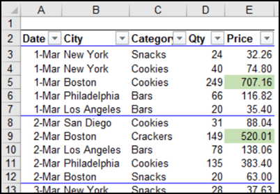
So in this table I have two rules.
–One puts a line at the top of a date, if it’s different from the date above.
–The other rule changes the price to green, if it’s greater than $500 dollars.
We’ll take a look at those rules. In the Home tab, go to Conditional Formatting, Manage Rules.
And there you can see the two rules. They’re each applied from row 3 to 19 in this table.
–Now this one is just a cell value greater than 500.
–And this one is referring to a couple of cells. So if A2 is different from A3, we’re going to put a blue line, at the top of the cell.
How Problems Happen
And now, I’m going to insert a row, because I forgot to put in one of the records here. So I’ll click, Insert. And then just put some data in this row.
So that was a simple change to the table. And now I’m going to go back and look at my conditional formatting rules again. And suddenly I have a new rule, just for the row that I inserted.
So row 11 has its own rule, and the previous rule is still there, going from A3 to E10, and then A12 to E20. So it’s skipping this row, because that row has a separate rule.
And if you insert lots of rows, you can end up with hundreds of these rules set up, without even knowing it.
The Solution
And what I do to fix it is select all the rows, except for the first one. Then go to Conditional Formatting, Clear Rules, From Selected Cells.
Now if I go back in, and Manage Rules…I’ll go back to This Worksheet, just so we can see everything. So we’re back to those two original rules.
Then, I select the first row. I’ll select the first row in the table, this time, instead of the whole worksheet.
And go to the Format Painter, and make sure you’re selecting this first row as well, and apply that formatting to all the rows again.
And when we go back to Manage Rules, we still just have those two original rules.
If you need to do this frequently, go to my website to get a macro that removes the duplicate rules. It’s designed for data in in an Excel named table.
End Of Transcript
Simple Conditional Formatting Rules
In this example, there is a small table, with 2 simple conditional formatting rules:
- In column E, highlight prices that are greater than 500
- In columns A:E, add a blue top border if the date in column A is different from the date above
New Rule Automatically Created
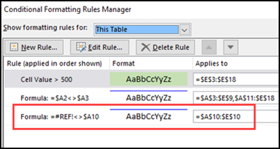
To see how a new rule is automatically created, delete row 10 in this table. Then, go to Conditional Formatting > Manage Rules, to see the results.
- The original rule has changed, and excludes the deleted row.
- There is a new rule that applies to row 10 only, and it has a #REF! error
Why It Happened
The new rule was created because the Top Border rule has a formula that refers to another row. It compares the date in the current row, to the date in the row above:
=$A2<>$A3
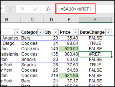
When you delete a row, the row below that loses its reference to that row. If we had the same formula on the worksheet, you’d see a #REF! error.
The same #REF! error occurs in the conditional formatting formula, so Excel creates a new rule for that formula.
Fix Conditional Formatting Duplicate Rules
If you frequently delete and insert rows, you could end up with many duplicated rules. In a big workbook, that could potentially slow down your workbook’s calculation speed.
And, you might not even know about those extra rules, unless you go into the Manage Rules dialog box for some reason.
I’ve written about this problem before, and there are a few ways to prevent the problem from occurring. Now that I’ve found an easy way to fix the problem, I don’t worry about prevention – I just clean things up when necessary.
Easy Steps to Fix the Problem
Here are the easy steps to remove the conditional formatting duplicate rules:
- Except for the first row, select all the rows with the same conditional formatting rules
- On the Excel Ribbon’s Home tab, click Conditional Formatting
- Click Clear Rules, then click Clear Rules from Selected Cells
- Select the first row, and on the Excel Ribbon’s Home tab, click the Format Painter
- Drag the Format Painter over all the cells where the conditional formatting rules should be applied, including the first row
To confirm that the duplicate rules were removed, go back to the Manage Rules window. Only the two original rules should be listed.
Get the Sample File and Macro
To get the sample file that I used in this example, go to the Conditional Formatting page on my Contextures website. The details are there, as well as the macro code. Scroll down a bit to see the link to download the file – it is in xlsx format, so the macro isn’t in that file.
________________


Bravo! This has brother me for years! Thank you!
Beautifully explained
I have seen the problem so many times and written code to re-apply formatting, but never fully understood what causes the issue in the first place.
Such an elegant, efficient, code-free solution.
I am in your debt, Ms Dalgliesh !
Thanks, Adam! I’m glad the article helped you with this annoying conditional formatting problem.
Thank you! Thank you! Thank you!
I’m another one that had this problem over and over.
Thanks
Thanks. I had so many duplicate rules that it took excel about 15 seconds to delete one of them. I got my duplicates when I copied and pasted. I realized that I had to copy and paste values to avoid this but I would often forget.
How to stop this Conditional Formatting. It irritating me as sometime not all info i need to do copy and paste with the same info. Please help if this can be switch off.
For the formula comparing to the row above, a better formula than $A2$A3 would be $A3OFFSET($A3,-1,0). This makes $A3 compare to one row above $A3. If you move row 2, delete row 2, or insert a new row between rows 2 and 3, the formula will continue to compare to whatever happens to be one row above it.
The clear all conditional formatting from all but one cell in the column, and then apply that cells formatting to everything else is a nice solution—thanks for that. It’s what I came here looking for. Now if there were only a way to build the conditional formatting in such a way that it wasn’t subject to proliferating new copies of the rules every time you copy or move rows .
Hello, Ms Dalgliesh.
First of all. Thank you for your code. Secondly. I copied your code to my Worksheet and tried to run the macro step by step using F8, and I am receiving this error from the second line line:
Set ws = Activesheet
Set MyList = ws.ListObjects(1) (Line of the error)
The exactly error of this Windows is:
Microsoft Visual Basic
Run-time error ‘9’:
Subscript out of Range
Continue End Debug Help
Any, recommendation for this error? I am very interesting in use this VBA in one of the my daily workbook.
Thank you for all your time.
Regards;
Carlos Peguero
Hi Carlos,
You need a table on your activesheet 🙂
In the code provided here, it seems that the existing format will be deleted (or replaced by format of row 1 of the table).
Is there a solution to only paste the conditional formatting ?
Thanks
GM, see my response below.
Your clear instruction and that macro is an absolute lifesaver! Thank you, thank you, thank you. This will save me a lot of time and general hair-pulling in the future. I really appreciate you making this free for people to learn.
You’re welcome, Nico, and thanks for letting me know that the macro helped you!
Debra, this elegant solution you describe here is fantastic. Thank you, it saved me literally hours cleaning up a spreadsheet with hundreds of conditional formatting remnants that were taking *minutes* each to delete.
I have an alternate suggestion to reestablishing the full conditional formatting range applying the format painter throughout the document, which could change other characteristics (such as a font size or text color unique to particular entries). Instead, the cell range over which the conditional formatting applies can be manually adjusted for each rule.
For example, my spreadsheet has six rules operating on the same range, which change cell colors depending on status text (Open, Closed, et al.). After clearing the all-but-first-row conditional formatting, the applicable range was =$B$4:$V$4. Editing $V$4 to $V$675 updated the range to cover all of my data without changing any other formatting.
Thanks, Dave, and you’re right – that method is much better if there is other formatting applied in the table.
Thank you so much. I had a spreadsheet with a full year of dates and names which had about 20 conditional formatting rules. With all the cutting and pasting that had been going on there literally hundreds and hundreds of rules that had duplicated. Your elegant solution was brilliant. I still had to delete the duplicate that had appeared in the first row, but that was simple compared to the alternative. From now on I will know how to manage these rules better. Thanks again!
You’re welcome, Bernadette, and thanks for letting me know that it helped you!
This touches on my issue, and I cannot see any way around manually fixing the format rule periodically. I have a column that is used for a unique list of IDs. The full list is pasted in, then duplicates are removed. That is where the cond format rule gets split up into pieces over time.
I tried using a Named Range, but it just parses that back into cell references. Any thoughts?