reach_whitepaper.md

Reach Implementation Best Practices in the Privacy Sandbox Shared Storage + Private Aggregation APIs

Authors: Hidayet Aksu ([email protected]), Alexander Knop ([email protected]), Pasin Manurangsi ([email protected])

This whitepaper aims to provide ad tech companies with actionable guidance on implementing reach measurement within the Privacy Sandbox, via the Shared Storage and Private Aggregation APIs. We dive into various reach scenarios, covering hierarchical queries, cumulative reach, and present corresponding implementation strategies, catering to diverse ad tech requirements.

In various use cases, we recognize the potential utilization of exploratory reach queries. Taking into account the various needs of advertising technology companies, we consider both scenarios: pre-determined reach queries (queries known in advance) and ad hoc or unknown reach queries. Hence, this work presents an exploration of alternative approaches, including direct measurement and sketch-based mechanisms. Through empirical evaluation on synthetically generated data, modeled after real-world ad datasets, we assess the impact of factors like ad event capping, query granularity, and time windows on measurement accuracy. We aim to equip ad tech companies with the insights needed to select the best reach measurement method aligned with their specific query characteristics and privacy considerations.

Our experiments show that for predetermined queries, the best solution is to use the point contribution mechanism. However for more exploratory queries or those with longer windows, sketch-based mechanisms are beneficial although techniques such as capping may need to be used to reduce error.

By shedding light on reach estimation using the Privacy Sandbox, this paper seeks to empower ad tech companies to navigate the evolving landscape of privacy-centric advertising technologies.

Reach Functionality

The goal of reach is to compute the number of unique users that see (or interact with) content (e.g., a specific ad). For the purpose of this white paper, we will treat each browser profile as a unique user, so that the result is actually the number of unique profiles that see the content. We use this definition for simplicity in our empirical evaluations. Therefore, we will use “user” and “browser profile” interchangeably.

In general, an ad tech would like to perform multiple reach measurements depending on how they wish to “slice” the set of users. In the context of digital advertising, a slice is defined as a distinct segment of a campaign's target audience, characterized by specific attributes or behaviors. This segmentation allows granular analysis and targeted optimization of advertising efforts. Slices can be constructed based on a variety of dimensions like campaign, location, demographics etc. For example, one may want to perform a reach measurement for a single campaign during a single day; or to perform a reach measurement for a single campaign during a single day for a specific geographic region.

Within a specified time window, reach between slices is not necessarily additive. In other words, the count of all users for campaign=123 is equal to the sum of user counts of campaign=123 for each geolocation, only if no user appears in two different geo areas, which is not always the case. For features such as a creative ID, a user may view advertisements with multiple creative IDs, thus additivity does not apply in this scenario either. Consequently, when queries are pre-determined, it is important to explicitly define each inquiry and collect relevant contributions. Conversely, when queries are unknown, contributions must be collected to support the finest granularity of queries.

Throughout this paper, we consider hierarchical reach measurement queries, based on different slices. For illustration and experimentation purposes, we assume the following four slicing levels:

• Level 1 (coarsest): advertiser
• Level 2: advertiser x campaign
• Level 3: advertiser x campaign x geo
• Level 4 (finest): advertiser x campaign x geo x ad strategy x creative

To analyze the temporal aspects of reach, let's consider the following definitions for a running campaign:

• Cumulative Reach: This quantifies the number of unique users exposed to impressions within a campaign since its inception. In this scenario, we incrementally measure reach over time.

  • Example queries: Reach until January 24th, Reach until January 25th, Reach until January 26th, etc.

  Note that we are not considering rolling window queries here for brevity; however, the approaches we consider for cumulative reach could be generalized to this use case.

• Fixed Window Reach: This calculates the number of unique users exposed to impressions within a specific time range. The time range, or window, is determined at the time of data collection and remains constant during subsequent analysis.

  • Example queries: Reach between January 22nd and January 24th, Reach between January 23rd and January 25th, etc.

  The following query examples were selected for pre-determined queries due to their relevance to real-world scenarios and frequent usage within ad tech analytics.

ID	Query	Query Frequency	Type
Q1	What is the reach for the last day?	Queried every day	Fixed Window
Q2	What is the reach for the last calendar week?	Queried every week	Fixed Window
Q3	What is the reach for the last month?	Queried every month	Fixed Window
QC	What is the cumulative reach till now?	Queried every day	Cumulative

Reach Implementations

First, we show that reach can be measured directly using the existing Shared Storage and Private Aggregation APIs – we call this approach a direct method. Next, we explain how sketch-based methods can be used with the same APIs.

Single Reach Measurement in Shared Storage + Private Aggregation APIs

We start by recalling how to compute a single reach measurement via Shared Storage, as described in the developer documentation. The idea is to use Shared Storage to record whether this browser has already contributed to the reach measurement for the slice. If it has, then we do nothing. Otherwise, we contribute to the histogram (with a single bucket) and record that a contribution has been made in Shared Storage. In doing so, the computed reach is simply equal to the aggregated value. For convenience, the following code snippet is adapted from the above linked documentation.

const L1_BUDGET = 65536;

// contentId here is some id of the interaction that is measured;
// i.e., it is a campaign id.
function convertContentIdToBucket(contentId) {
  return BigInt(contentId);
}

class ReachMeasurementOperation {
  async run(data) {
    const { contentId } = data;

    // Read from Shared Storage
    const key = 'has-reported-content';
    const hasReportedContent = (await sharedStorage.get(key)) === 'true';

    // Do not report if a report has been sent already
    if (hasReportedContent) {
      // Note that this would happen if less than 30 days 
      // passed since the first visit.
      return;
    }

    // Generate the aggregation key and the aggregatable value
    const bucket = convertContentIdToBucket(contentId);
    const value = 1 * L1_BUDGET;

    // Send an aggregatable report via the Private Aggregation API
    privateAggregation.contributeToHistogram({ bucket, value });

    // Set the report submission status flag
    await sharedStorage.set(key, true);
  }
}

Note that the reach result can be computed by taking the aggregated histogram value of each key and dividing by the contribution budget (L1_BUDGET). Note that the developers website uses a scale factor (SCALE_FACTOR), but in this example the scaling factor is the same as the contribution budget so we use L1_BUDGET. See the “Noise and scaling” section of the Private Aggregation fundamentals article to learn more.

Single Reach Measurement with Capping

An implicit assumption in the previous section is that each privacy unit – i.e., <browser x reporting origin ad tech x 10 minutes> – contributes to only a single query. The reason is that (i) the Shared Storage check does not incorporate the bucket so even if a later content tries to contribute to the same report, it will not pass the check and (ii) the value contribution is 65,536 which is the same as the overall contribution budget (see contribution budget for summary reports). In other words, we “cap” the number of contributions each privacy unit can make to just one. In many cases, multiple contributions from a single privacy unit may be dropped due to a capping limit of 1. This can lead to poor utility, as each privacy unit's contributions are not fully reflected in the results.

To improve utility, we can increase the contribution cap to an arbitrary number we wish (denoted by CONTRIBUTION_CAP below). Allowing a larger cap can capture more contributions, which is good for utility. However, it also results in a larger amount of noise (after scaled down by L1_BUDGET / CONTRIBUTION_CAP) which is worse for utility. As such, the capping parameter has to be tuned carefully.

We give an example code below where the capping parameter is set to five. The two changes are (i) making the Shared Storage checks for the specific bucket and (ii) dividing each contribution value by the capping parameter. These changes are highlighted in light yellow.

const CONTRIBUTION_CAP = 5;
const L1_BUDGET = 65536;

function convertContentIdToBucket(contentId) {
  return BigInt(contentId);
}

class ReachMeasurementOperation {
  async run(data) {
    const { contentId } = data;

    // Generate the aggregation key and the aggregatable value
    const bucket = convertContentIdToBucket(contentId);
    const value = Math.floor(L1_BUDGET / CONTRIBUTION_CAP);

    // Read from Shared Storage
    const key = `has-reported-content-${bucket}`;
    const hasReportedContent = (await sharedStorage.get(key)) === 'true';

    // Do not report if a report has been sent already for this bucket
    if (hasReportedContent) {
      return;
    }

    // Send an aggregatable report via the Private Aggregation API
    privateAggregation.contributeToHistogram({ bucket, value });

    // Set the report submission status flag
    await sharedStorage.set(key, true);
  }
}

Multiple Reach Measurements with Capping

While the above method focuses on a scenario where each content can contribute to only a single reach measurement (i.e., a single “query”), it can be extended to the case where each content can contribute to multiple reach measurements by having a key for each query.

Below, we give an example of this for the hierarchical queries described above. Note that each reached browser (i.e., first time the advertisement is shown to the user) contributes to exactly one slice in each level. Thus, the number of histogram keys that each reached content contributes to is equal to the number of levels. Due to the contributions budget constraint, the scale factor is now divided by the number of levels in addition to dividing it by the contribution cap (CONTRIBUTION_CAP). While we adhere to equal contribution per level, it is possible to further optimize the contribution budget across different levels, as explained in the relevant paper.

The code for this is below.

const CONTRIBUTION_CAP = 5;
const NUM_LEVELS = 4;
const L1_BUDGET = 65536;

function convertContentIdAndLevelToBucket(contentId, level, ...otherDimensions) {
  // Implement a function that computes the bucket key for a given level using 
  // level-related fields from otherDimensions.
  // E.g., in our example, the second level could set the key to be the concatenation
  // between advertiser and campaign id of this content.
}
class ReachMeasurementOperation {
  async run(data) {
    const { contentId, ...otherDimensions } = data;

    for (let level = 1; level <= NUM_LEVELS; level++) {
      // Generate the aggregation key and the aggregatable value
      const bucket = convertContentIdAndLevelToBucket(contentId, level, ...otherDimensions);
      const value = Math.floor(L1_BUDGET / (CONTRIBUTION_CAP * NUM_LEVELS));

      // Read from Shared Storage
      const key = `has-reported-content-${bucket}`;
      const hasReportedContent = (await sharedStorage.get(key)) === 'true';

      // Do not report if a report has been sent already
      if (hasReportedContent) {
        return;
      }

      // Send an aggregatable report via the Private Aggregation API
      privateAggregation.contributeToHistogram({ bucket, value });

      // Set the report submission status flag
      await sharedStorage.set(key, true);
    }
  }
}

// Register the operation
register('reach-measurement', ReachMeasurementOperation);

A sample call would look like:

await window.sharedStorage.run('reach-measurement', { data: {
    contentId: '123', 
    geo: 'san jose', 
    creativeId: '55' 
}});

Cumulative Reach Measurements

So far, we have not mentioned the time aspect of the queries. In particular, we assume that all queries correspond to the same time periods. However, we may want to measure time-related queries. A popular family of such queries is cumulative queries, which are queries of the form “what is the total reach up until timestep t?” where t varies from 1, …, T. For example, one might want to measure the reach up until today everyday for the entire month. In this case, we would have T = 30 and “timestep” being a day.

Note: Both methods described in this section are limited by the retention policy of Shared Storage which is 30 days from last write.

Direct Method

For cumulative reach queries, we can naively apply the direct method above by adding the timestamp to the key of the histogram. If a user is reached at time step $i$, then contributions would be made to all of $i, \dots, T$ buckets. Since there are $T$ queries, the noise will scale by a factor of $O(T / \epsilon)$. Note that with the current API, one would need to wait until the last window to obtain the results since reprocessing of the reports is not currently supported.

Point Contribution

We can improve upon the above direct method by a simple modification. For simplicity, we only discuss the mechanism (and give the code) for the single-query cap-one case. It is easy to extend this to the multi-query case by appending the query id to the keys. Before we describe the mechanism, let us first make the following observation. Consider the number $n^{(\text{new})}_i$ of users that were reached for the first time at timestep $i$. The answer of cumulative reach up to timestep $t$ is exactly equal to the cumulative sum $\sum\limits_{i=1}^t n^{(\text{new})}_i$. Using this fact, we can simply create $T$ buckets, where bucket $i$ corresponds to $n^{(\text{new})}_i$. When we wish to compute the cumulative reach up to time step $i$, we take the sum of the first $i$ buckets. Since each user contributes to only a single bucket, each bucket’s noise standard deviation is only $O(1 / \epsilon)$. Since we are summing up to $T$ such (independent) noises, the total noise standard deviation is $O(\sqrt{T} / \epsilon)$, which is an improvement of $O(\sqrt{T})$ over the direct method.

An implementation in Shared Storage is given below.

// Time horizon T
const TIME_HORIZON = 30;
const L1_BUDGET = 65536;

function convertContentIdToBucket(contentId, currentTime) {
  // This key corresponds to n_i as described above with i = currentTime.
  // Note that the remainder of "bucket" when divided by TIME_HORIZON
  // is currentTime and the quotient is contentId; hence, this formula gives a 
  // unique id to each pair of contentId and currentTime.
  return TIME_HORIZON * BigInt(contentId) + currentTime;
}

class ReachMeasurementOperation {
  async run(data) {
    const { contentId } = data;

    // Read from Shared Storage
    const key = 'has-reported-content';
    const hasReportedContent = (await this.sharedStorage.get(key)) === 'true';

    // Do not report if a report has been sent already
    if (hasReportedContent) {
      return;
    }

    // Should be appropriately set by the ad tech (e.g., based on hour or day)
    const currentTime;
  
    // Increment the current bucket
    const bucket = convertContentIdToBucket(contentId, currentTime);
    const value = L1_BUDGET;

    // Send an aggregatable report via the Private Aggregation API
    privateAggregation.contributeToHistogram({ bucket, value });

    // Set the report submission status flag
    await this.sharedStorage.set(key, true);
  }
}

The code for computing cumulative reach from the aggregated histogram is given below.

# Time horizon T; needs to be fixed beforehand
TIME_HORIZON = 30;
L1_BUDGET = 65536.0;


def convert_content_id_to_bucket(content_id: int, current_time: int) -> int:
    # Same as the client-side function above.
    return TIME_HORIZON * content_id + current_time;

def compute_cumulative_reach(
    aggregated_histogram: dict[int, int],
    content_id: int) -> dict[int, int]:
  """Compute cumulative reach for the given content_id.

  Args:
    aggregated_histogram: a mapping from key to aggregated value n the summary 
      report output by the Aggregation Service.
    content_id: the content id for which the cumulative reach is computed.

  Returns:
    a mapping from time step to the cumulative reach up until that time step.
  """
  res = {}
  for t in range(TIME_HORIZON):
    res[t] = 0
    for i in range(1, t + 1):
      key = convert_content_id_to_bucket(content_id, i)
      res[t] += aggregated_histogram[key] / L1_BUDGET
  return res

Finally, we remark that, for larger values of T (which may be the case if measuring cumulative reach on granularities less than one day), there are more advanced mechanisms that can reduce the error further [1,2], but this is beyond the scope of this paper.

Sketch-Based Methods

Sketching is a technique for estimating the reach (and other quantities of interest) using compressed aggregated data structure admitting merge operation. Here we only consider one of the most basic families of sketches, called counting bloom filters (CBFs). In this case, we have a hash function $h$ that maps any user ID to one of $m$ buckets. The CBF sketch is simply the histogram on these $m$ buckets among all the reached users. We can estimate the reach based on the number of non-empty buckets in the sketches. The exact formula for this estimation is based on the hash function distribution.

The main advantage of this sketch is that it can be merged: if we have two CBFs, summing them up gives us the CBF corresponding to the union of the two (multi)sets. This allows us to be more flexible when answering queries. Recall that, in the direct method, we need to know all the queries beforehand since we need to allocate each bucket and each query. This is not needed when using sketches: We can simply create a sketch for each fine-grained unit (e.g. the reach for each day) and, when we make a query for a day range, we take the union of all the sketches in that range. This means that the analyst can supply the queries in an on-demand fashion, which is more convenient. Moreover, sketching methodology offers another significant advantage: the ability to deduplicate user IDs across multiple devices, providing a more accurate picture of individual engagement. This would typically require using the same user ID on multiple devices. Shared Storage is partitioned per browser, so the ad tech would need to identify the user across devices independently. Alternatively, there are modeling-based approaches (e.g. virtual people) that would avoid the need for these IDs to map directly to real-world users.

Nevertheless, there are also several disadvantages of this sketch. Firstly, each sketch is a histogram with $m$ buckets. In contrast, the direct method only outputs a single number per query. Therefore, the sketching method can result in a memory usage overhead during processing of the aggregatable reports and during post-processing of the summary reports compared to the direct or point contribution methods. Secondly, since the noise is added to every entry of the sketch, this can lead to inaccurate estimates if the noise is large. Specifically, as we will see below, we need to set the capping parameter to be small to ensure the noise is small but doing so results in a large error due to capping. This tension means that we have to be very careful in terms of parameter settings to ensure (reasonably) accurate estimates.

The overall scheme of the reach estimation involving sketches is described on the following diagram.

We remark that there are many other types of sketches beyond counting bloom filters (CBFs), such as (boolean) bloom filters; and even CBF’s could use different hashes with different distributions of values. In this paper, we only focus on uniform CBFs since they are histograms and thus most compatible with the API and change of the distribution didn’t change the experimental errors in our dataset. However, it is plausible that other types of sketches can allow for better utility.

As the sketch is simply a histogram, it is simple to implement via the Shared Storage and Private Aggregation APIs. Again, for simplicity, we only include the code snippet for the cap-one case below. (Note that if there are many different content ids, one might consider splitting them into groups using filtering ID’s.)

// Sketch size m
const SKETCH_SIZE = 10000
const L1_BUDGET = 65536;

function sketchHash(userId) {
  // Should output a number in 0, ..., SKETCH_SIZE - 1 based on which bucket of 
  // the sketch the user id is hashed to.
}

function convertContentIdToBucket(contentId, userId) {
  // Note that the remainder of convertContentIdToBucket when divided by 
  // SKETCH_SIZE is sketchHash(userId) and the quotient is contentId; hence, 
  // this formula gives a unique id to each pair of contentId and 
  // sketchHash(userId).
  return SKETCH_SIZE * BigInt(contentId) + sketchHash(userId);
}

class ReachMeasurementOperation {
  async run(data) {
    const { contentId } = data;

    // Read from Shared Storage
    const key = 'has-reported-content';
    const hasReportedContent = (await sharedStorage.get(key)) === 'true';

    // Do not report if a report has been sent already
    if (hasReportedContent) {
      return;
    }

    // Generate the aggregation key and the aggregatable value
    const userId = getUserId();
    const bucket = convertContentIdToBucket(contentId, userId);
    const value = 1 * L1_BUDGET;

    // Send an aggregatable report via the Private Aggregation API
    privateAggregation.contributeToHistogram({ bucket, value });

    // Set the report submission status flag
    await sharedStorage.set(key, true);
  }
}

After aggregation, each content id will have a sketch associated with it. To estimate the reach given sketches the following algorithm can be used.

import numpy as np

def _invert_monotonic(
    f: Callable[[float], float], lower: float = 0, tolerance: float = 0.001
) -> Callable[[float], float]:
    """Inverts monotonic function f."""
    f0 = f(lower)

    def inversion(y: float) -> float:
        """Inverted f."""
        assert f0 <= y, (
            "Positive domain inversion error."
            f"f({lower}) = {f0}, but {y} was requested."
        )
        left = lower
        probe = 1
        while f(probe) < y:
            left = probe
            probe *= 2
        right = probe
        mid = (right + left) / 2
        while right - left > tolerance:
            f_mid = f(mid)
            if f_mid > y:
                right = mid
            else:
                left = mid
            mid = (right + left) / 2
        return mid

    return inversion

def _get_expected_non_zero_buckets(
   bucket_probabilities: list[float],
) -> Callable[[int], float]:
   """
   Create a function that computes the expected number of non-zero buckets.

   Args:
       bucket_probabilities: A list of probabilities of each bucket
           being selected when a user is added to a sketch.
   Returns:
       A function that given the number of users, returns the expected number of
       non-empty buckets.
   """
   def internal(count: int):
       return sum(
                1 - pow(1 - p, count)
                for p in bucket_probabilities
            )
   return internal


def estimate_reach(
    sketches: list[list[int]], 
    bucket_probabilities: list[float],
) -> float:
    """
    Estimate reach given the sketches.

    Args:
        sketches: the list of sketches, where each element of a sketch is an 
            element of the histogram.
        bucket_probabilities: probability of a given bucket being chosen for a
            user; for uniform CBF's all the values are the same, for exponential
            CBF ith element has value `alpha ** i` for some fixed value alpha.
    """
    sketches = np.array(sketches)
    
    thresholded_sketches = (sketches >= 0.5).astype(int)
    merged_sketch = thresholded_sketches.sum(axis=0)
    thresholded_merged__sketch = (merged_sketch >= 0.5).astype(int)
    non_zero_buckets_count = thresholded_merged__sketch.sum()

    estimator = _invert_monotonic(
        _get_expected_non_zero_buckets(bucket_probabilities), 
        lower=0, 
        tolerance=1e-7,
    )

    return estimator(non_zero_buckets_count)

Empirical Evaluation

Data

Due to privacy concerns, in this paper, we choose to evaluate errors on synthetic data. Working on real ad datasets, we find out that the reach on datasets can be modeled in the following way. Reach for one day follows power-law distribution with shape parameter $b$. When analyzing different datasets based on the different query or various slice definitions, such as hierarchical queries, we noticed a consistent pattern. Specifically, these datasets exhibit a power-law distribution, albeit with differing shape parameters. In our observations, it was noted that capping on the client side does not affect the shape of the power-law distribution, indicating that campaign impressions are dropped by capping with equal probability. In contrast, capping does have a significant impact on the volume reports from clients. The rate of reports dropped by capping, i.e., the capping discount rate, follows a power-law distribution with respect to the capping value. Figure 2 displays a representative discount rate versus capping plot and corresponding curve fitting.

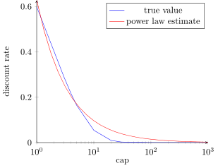
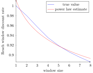
Furthermore, we examined the impact of the time window on the reach. Reach does not demonstrate a linear relationship with time window size. Instead, it exhibits a diminishing return compared to linear growth as illustrated in Figure 3. This discount follows a power-law function relative to the size of the time window.

def sample_slices(
   number_of_days,
   cap,
   dataset_power_law_shape,
   n_samples
) -> list[SliceSize]:
"""Generates a synthetic dataset in slices (tuples of capped and uncapped numbers).


 Args:
   number_of_days: what time window the query is using.
   cap: the maximal number of slices a user might contribute.
   dataset_power_law_shape: dataset specific power-law shape param.
   n_samples: number of slices to generate. 
 """


  # sample reach distribution from power-law distribution. 
  reach_1_day = sample_discrete_power_law(
    b=dataset_power_law_shape, 
    n_samples=n_samples,
    ...)
  # approximate impact of capping.
  # compute probability of being reported (success, not impacted by capped) 
  # after capping.
  p_reported = (1 - cap_discount_rate(cap=cap))
  # for a slice of true size n, each contribution has p_reported probability to
  # be reported. Thus after capping, observed contributions become 
  # np.random.binomial(n, p) (there may be faster approximations) 
  reach_1_day_capped =  np.random.binomial(reach_1_day, p_reported)


  # approximate impact of time window
  reach_n_days = reach_1_day * number_of_days * window_discount_rate(number_of_days)
  reach_n_days_capped = reach_1_day_capped * number_of_days * window_discount_rate(number_of_days)


  # round to nearest int 
  reach_n_days = np.round(reach_n_days).astype(int)
  reach_n_days_capped = np.round(reach_n_days_capped).astype(int)


  return [
    (uncapped, capped) 
    for uncapped, capped in zip(reach_n_days, reach_n_days_capped)
  ]

Listing 1: pseudocode to generate synthetic data.

Level (granularity)	Query dimensions	Power law shape (b) param # reach per bucket
1 (coarsest)	advertiser	1.01
2	advertiser x campaign	1.10
3	advertiser x campaign x geo	1.50
4 (finest)	advertiser x campaign x geo x ad strategy x creative	1.60

Table 2: shape params used in experiments for queries with different granularity.

In accordance with the pseudocode presented in Listing 1, synthetic datasets of variable sizes, capping values, and time windows were generated for experimental evaluation.

Error Metrics

In our experiments we are going to use $\text{RMSRE}_\tau$ metric defined as follows:

$$\mathrm{RMSRE}_\tau\left(\{t_i\}_{i = 1}^n, \{e_i\}_{i = 1}^n\right) = \sqrt{\frac{1}{n} \sum\limits_{i=1}^n \left(\frac{t_i - e_i}{\max(\tau, t_i)}\right)^2},$$

where $\{t_i\}_1^n$ are true values that we’d like to measure, and $\{e_i\}_1^n$ are the estimates.

Experimental Evaluation

As it was mentioned the data used in the experiments is synthetically generated. W e perform four experiments:

1. First, we measure the error introduced by capping.
2. Next, we measure the error (for each granularity level and three different windows: one day, one week, and one month).
3. In addition, we measure the error of the cumulative queries with and without the point contribution mechanism.
4. Finally, we examine the error of sketching-based methods.

Results

Error Caused by Capping

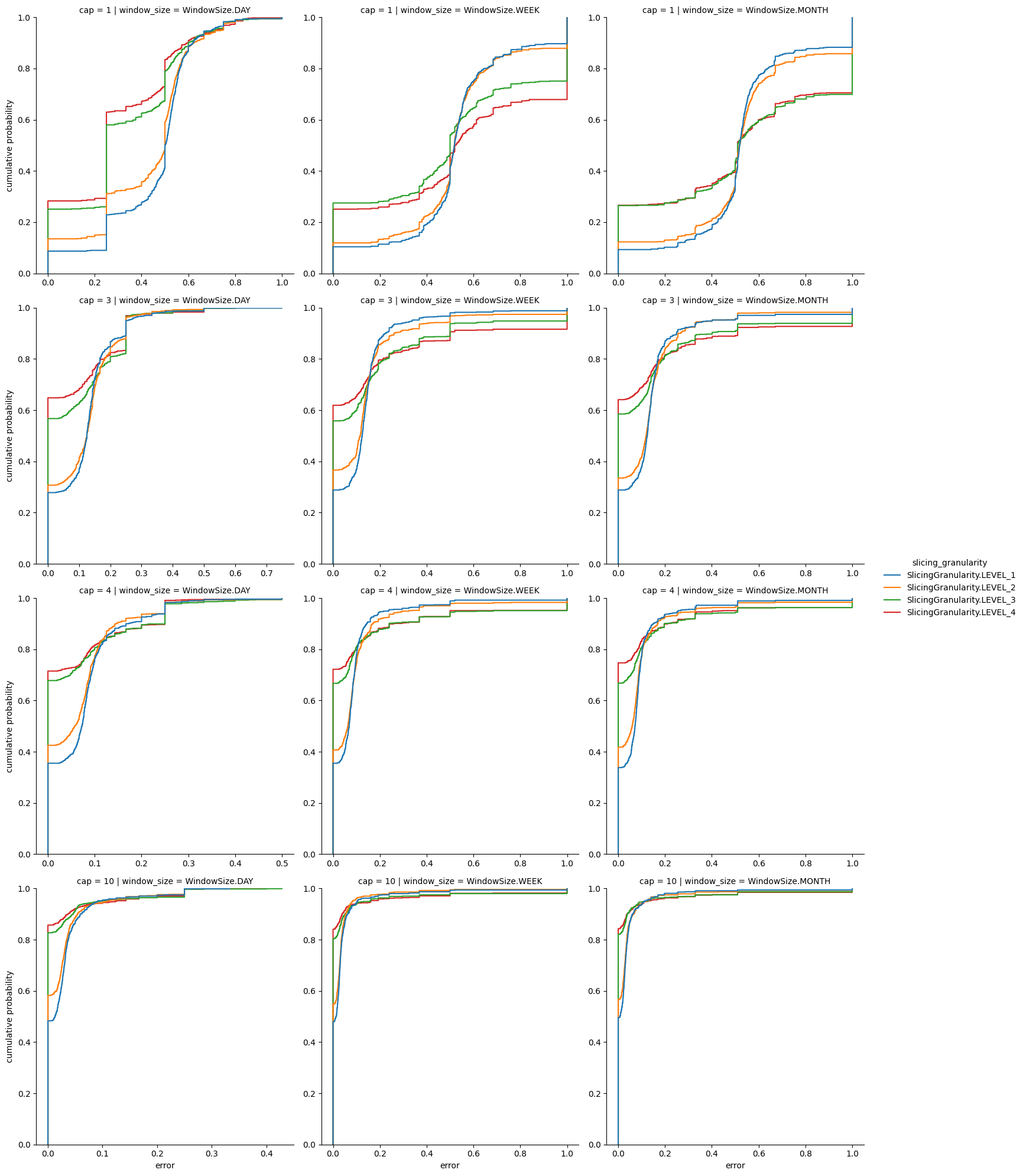
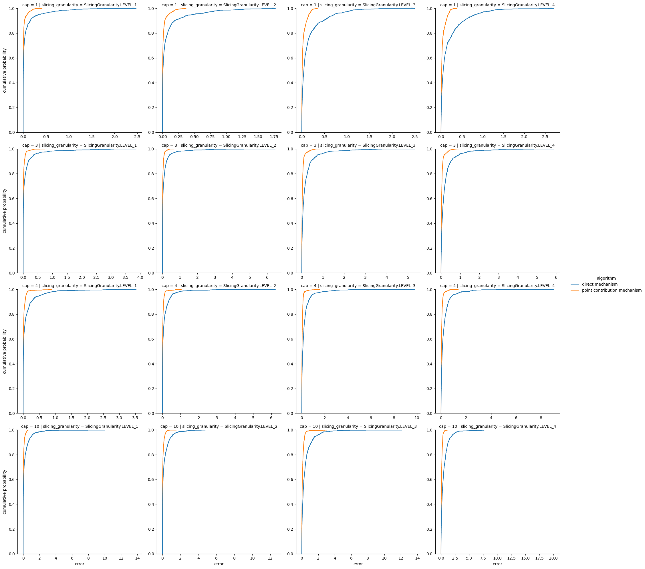
To measure the error caused by capping, we sampled 1000 samples of slices for each size of the window (1 day, 7 days, 30 days) and each granularity of the query, and computed $\text{RMSRE}_\tau$ error where the estimated value is true observed value (before adding noise or using sketches).

Next we plot the fraction of the samples with the error below t vs t. The plot shows that to achieve an error of at most 0.1 with probability at least 80%, we need to choose the capping to be at least 4.

Multiple Reach Measurements

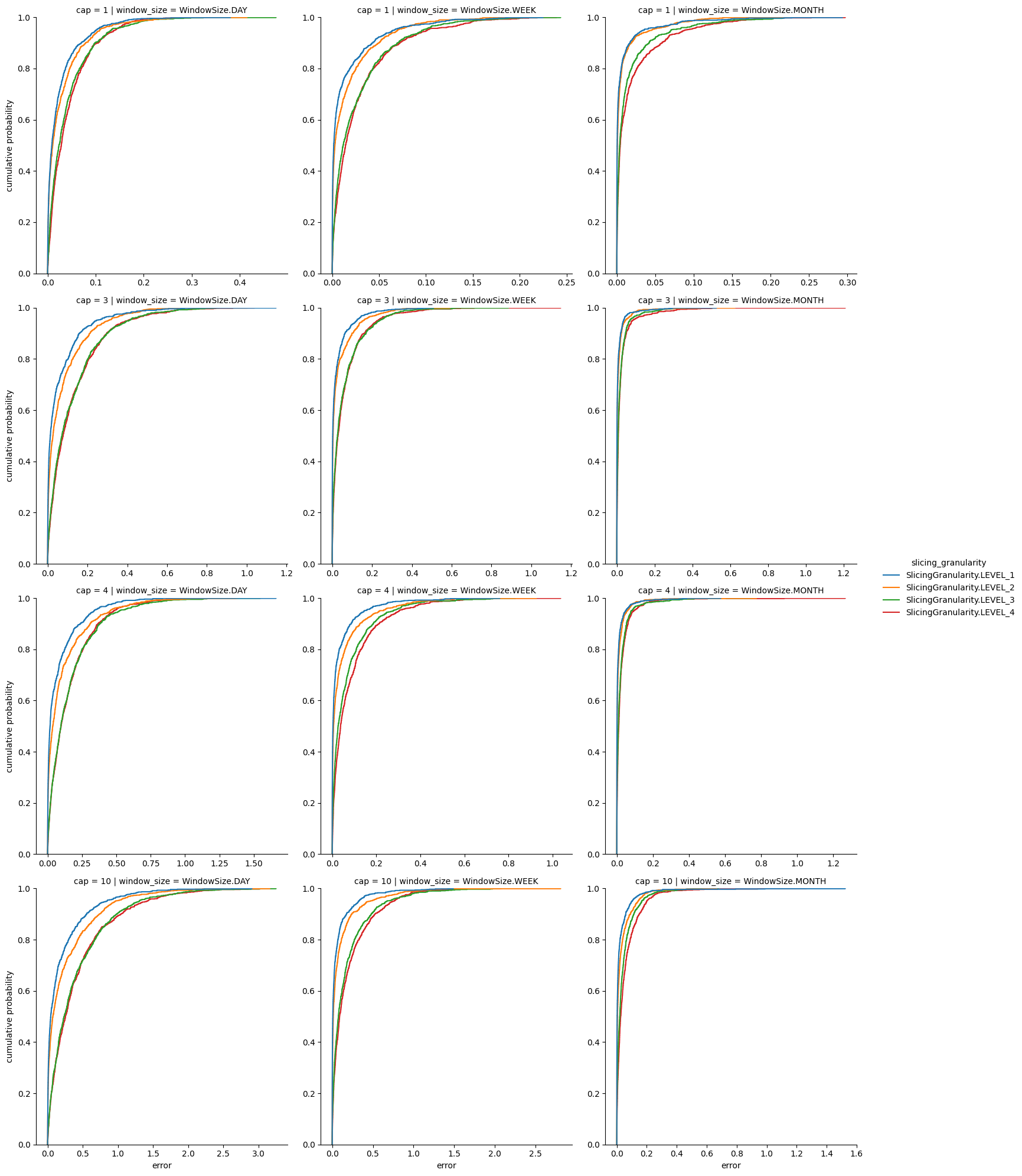
To measure the error introduced by noise in case of multiple measurements, we sampled 1000 slices for each size of the window (1 day, 7 days, 30 days) and each granularity of the query. Next we computed $\text{RMSRE}_\tau$ error where the true value is true observed value and estimated value is the noised observed value.

Next, we plot the fraction of the samples with the total error below t vs t, i.e. the error including both capping and noise. The plot shows that if we want to measure at least the week window, error less than 0.1 can be achieved for all granularities, and for the coarsest one error less than 0.05 can be achieved for cap equal to 4 with probability 80%, for window size of a month even for cap equal to 10 the error 0.1 can be achieved for all granularities with probability at least 80%, finally, for window size of a day, the error 0.1 with probability 80% is only achievable for cap equal to 1.

Cumulative Reach Method Error

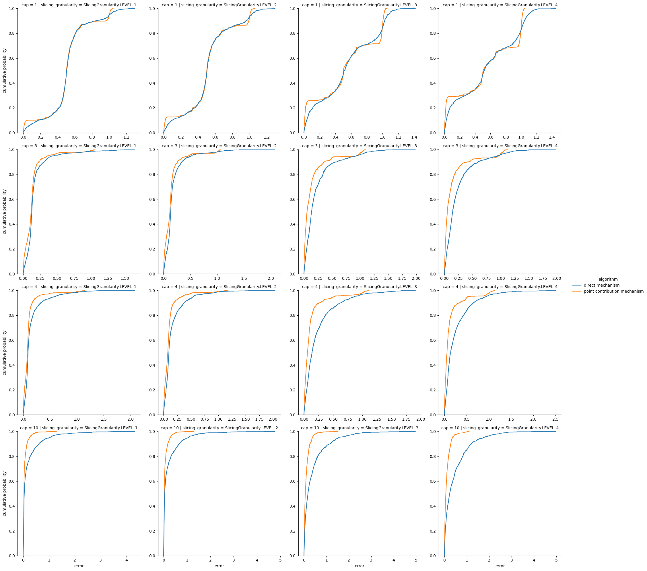
To measure cumulative reach, one can simply use the approach described above (i.e., using direct method); however, as it was mentioned before, point contribution mechanism adds noise with smaller standard deviation.

To show that this indeed provides better utility in the applications we plot the fraction of the samples with the total error on the last day (i.e., on the 30th day) below t vs t. As one may see from the plots, values of cap where observation error is not too large, the point contribution method gives sufficient improvement over the direct method and should be used for cumulative queries.

Sketch Method Error

For the last experiment, for window sizes of 1, 10, 20, …, 360 days we sampled 100 slices and computed the $\text{RMSRE}_\tau$ error where the true value is true observed value and estimated value is obtained from sketches of size 10000 (sketches need to be big to accommodate a year worth of data). Note that for each window size, we assume that reach is distributed uniformly across the window.

We plot the window size vs the total error and the shade denotes the 80% probability band. As it can be seen the error is somewhat stable and for a cap larger than 3 the error is too high; however, for a cap equal to 3 the median error is around 0.1 and stays within 0.2 with probability of 80%.

Conclusion

Our experiments show that if the query is pre-determined and the window is less than 30 days, the best solution would be to use the point contribution mechanism. However, if the queries are not determined at the collection time and/or the necessary window is over 30 days then the sketch method can be used; but it is important to limit the cap used to smaller values since otherwise the error is too high. The relatively large (compared to direct method) decrease in utility of the sketching method is due to the addition of noise to each intermediate sketch before the final result is computed. This could be addressed with evolution of the API design to allow ad techs to perform queries on sketches and only add noise to the final result.

We are hopeful that this paper will enable advertising technologists to comprehend the trade-offs associated with various methodologies and develop a structured path to implementing reach using the APIs.

For the implementation of experimental evaluations, please refer to the evaluation code.

Acknowledgements

We would like to thank Badih Ghazi, Charlie Harrison, Ravi Kumar, Asha Menon, and Alex Turner for their input and help with this work.

References

1. ​​Jean Bolot, Nadia Fawaz, S. Muthukrishnan, Aleksandar Nikolov, Nina Taft:_ Private decayed predicate sums on streams_. ICDT 2013: 284-295
2. Badih Ghazi, Ravi Kumar, Jelani Nelson, Pasin Manurangsi: Private Counting of Distinct and k-Occurring Items in Time Windows. ITCS 2023: 55:1-55:24
3. Cynthia Dwork, Moni Naor, Toniann Pitassi, Guy N. Rothblum: Differential privacy under continual observation. STOC 2010: 715-724
4. T.-H. Hubert Chan, Elaine Shi, Dawn Song: Private and Continual Release of Statistics. ICALP (2) 2010: 405-417
5. Cynthia Dwork, Moni Naor, Omer Reingold, Guy N. Rothblum: Pure Differential Privacy for Rectangle Queries via Private Partitions. ASIACRYPT (2) 2015: 735-751
6. Joel Daniel Andersson, Rasmus Pagh: A Smooth Binary Mechanism for Efficient Private Continual Observation. NeurIPS 2023