With its vast array of features, Excel is the go-to tool for data analysis, reporting, and everyday business tasks. As you deal with extensive datasets, it becomes crucial to maintain a clear view of your headers or specific data points. One feature that becomes indispensable in such situations is the ability to freeze rows.
Freezing rows in Excel is akin to having a stationary header while scrolling through a newspaper. Imagine scrolling down a massive list and losing track of which column represents which data type. Annoying, right? That’s where the magic of freezing comes into play. It allows you to keep certain rows visible, typically the headers, while navigating through your dataset. It ensures clarity, especially when working with large datasets.
Try implementing an automated software solution to enhance financial management and avoid manual data entry errors and loss – give Synder a try.
Understanding the concept of “freezing” in Excel
Before we delve deep into ways of freezing rows and columns in Excel, it’s essential to understand the concept. When you lock a row or column, you literally freeze them in place. This is different from splitting, where the Excel worksheet divides into separate panes. Each pane scrolls separately, but frozen rows or columns remain constant across the worksheet.
The primary scenario for freezing rows is when you have headers in Excel. By freezing headers, even if you scroll down a thousand rows, the header remains visible, providing context to the data you’re viewing.
Guide to freezing a row in Excel
In Excel, you can easily freeze (or lock) rows and columns to keep them visible as you scroll through the rest of the worksheet. Here’s how to freeze rows and columns in Excel:
How to freeze a row or column in Excel desktop version:
1. Open your Microsoft Excel workbook.
2. Navigate to the row in Excel or column you want to freeze.
- If you wish to freeze only the top row, you don’t need to select it specifically.
- If you want to freeze more than one row or column, select the row or column after the last one you want to freeze. For instance, if you wish to freeze the first three rows, click on the row number 4.
3. Go to the View tab on the ribbon at the top of Excel.
4. Locate the “Window” group. Here, you’ll find the option for freezing panes. Click on “Freeze Panes” to see a drop-down menu with three options:
- Freeze Top Row: This freezes the first row of the spreadsheet.
- Freeze First Column: This freezes the first column of the spreadsheet.
- Freeze Panes: Use this option to freeze more than one row or column. This will lock rows above your current selection and columns to the left of your current selection.
5. Choose the appropriate option for your needs and select freeze.
To unfreeze:
1. Go back to the View tab in the ribbon.
2. Click on “Freeze Panes” in the “Window” group.
3. From the dropdown, select “Unfreeze Panes.”
For Excel Online:
The process is slightly different.
1. Open your Excel spreadsheet.
2. Highlight the row or column you want to freeze.
3. Right-click to bring up the context menu.
4. Find and select the option to freeze the row or column.
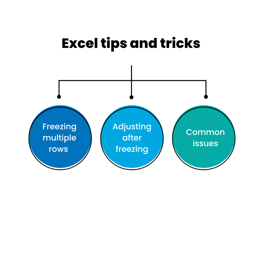
Tips and tricks
Now that you’ve learned how you can freeze the rows in Excel, here are some additional insights:

Freezing multiple rows or columns
If you want to freeze more than one row or column, select all the rows or columns you wish to freeze, then follow the same steps.
Adjusting after freezing
Once a row is frozen, the rest of the sheet scrolls while the frozen row remains in place. Adjust the row heights or column widths if any formatting issues arise.
Common issues
If you can’t freeze a row, ensure that you haven’t split the sheet. If split, remove the split first before freezing.
Learn the essential Excel formulas for accounting – read the article.
Conclusion
Mastering the art of freezing rows in Excel is a game-changer, especially for those regularly working with extensive datasets. By ensuring your headers or crucial data points remain visible, you enhance data comprehension and streamline data analysis.
FAQ section
Can I freeze rows and columns simultaneously?
Yes. If you want to freeze both rows and columns, select the cell that’s immediately below the rows and to the right of the columns you wish to freeze. Then, choose “Freeze Panes”.
Why can’t I see the “Freeze Panes” option in my Excel?
If you’re using Excel for the web (Excel Online), the “Freeze Panes” option might not be available in the same manner as in the Excel desktop application. The functionality and appearance might vary depending on the version of Excel you’re using.
What happens to formulas when a row is frozen?
Freezing doesn’t affect the functionality of formulas. They work as they typically would.
Is there a shortcut key to freeze rows in Excel?
While there isn’t a direct keyboard shortcut to freeze rows, you can use the Alt keys in sequence. For instance, pressing Alt + W, followed by F and then R, will freeze the top row.
Can I freeze rows in the middle of the sheet, leaving both the top and bottom sections scrollable?
No, when you freeze rows, only the section below the frozen rows becomes scrollable. The rows above remain stationary.
Read mor about How to create a pivot table in Excel and How to merge cells in Excel.


