Abstract
Pulmonary interlobar fissures are important anatomic structures in human lungs and are useful in locating and classifying lung abnormalities. Automatic segmentation of fissures is a difficult task because of their low contrast and large variability. We developed a fully automatic training-free approach for fissure segmentation based on the local bending degree (LBD) and the maximum bending index (MBI). The LBD is determined by the angle between the eigenvectors of two Hessian matrices for a pair of adjacent voxels. It is used to construct a constraint to extract the candidate surfaces in three-dimensional (3D) space. The MBI is a measure to discriminate cylindrical surfaces from planar surfaces in 3D space. Our approach for segmenting fissures consists of five steps, including lung segmentation, plane-like structure enhancement, surface extraction with LBD, initial fissure identification with MBI, and fissure extension based on local plane fitting. When applying our approach to 15 chest computed tomography (CT) scans, the mean values of the positive predictive value, the sensitivity, the root–mean square (RMS) distance, and the maximal RMS are 91 %, 88 %, 1.01 ± 0.99 mm, and 11.56 mm, respectively, which suggests that our algorithm can efficiently segment fissures in chest CT scans.
Keywords: Fissure segmentation, Chest CT data, Local bending degree, Maximum bending index, Local plane fitting
Introduction
An interlobar fissure consists of a double layer of visceral pleura and is generally 1–3 mm thick [1]. The right lung is divided into three lobes by an oblique fissure and a horizontal fissure, whereas the left lung is divided into two lobes by an oblique fissure. Detection of fissures is an important procedure in lung registration and lobe segmentation, which is useful to surgical intervention planning, and is helpful for locating lung abnormalities in computer-aided diagnosis systems. Although fissures can be easy for the radiologists to pick out instantaneously on their own, automatic fissure detection is still a challenging task.
To date, some semiautomatic and fully automatic fissure detection methods have been reported in the literature, which could be classified into three types: two-dimensional (2D) methods [2], 2D and three-dimensional (3D) hybrid methods [3, 4], and true 3D methods [5–9]. The former two methods mainly employed 2D operators, such as VanderBrug linear feature detector [2] and shape-based curve-growing model [3, 4], to detect fissures slice by slice. Then, different 2D and 3D methods were used to mend the segmented fissures. Due to the discontinuity of fissures in 2D space and the lack of 3D information in the 2D methods, human intervention was expected [3, 4] or some fissure patches were missing [2]. Compared to these methods, 3D methods [5–8] performed better. Because pulmonary fissures have a planar shape in 3D computed tomography (CT) images, the computational geometry theory [5] and the eigenvalues of the Hessian matrix [6–8] were employed to detect fissures. But the eigenvalues of the Hessian matrix cannot distinguish fissures from the walls of other tissues, so extra processing was required. For instance, several supervised filters constructed through training were used to segment the fissures [6, 8]. Although they achieved good performance, they required a significant amount of workloads for manual segmentation of fissures and long computational time to train the system. Gu et al. [9] developed a plane fitting algorithm to identify the planar patches and then classified them into three types of fissures.
We proposed a fully automatic training-free algorithm for segmenting fissures on chest CT volume data. Our method is based on the observation that fissures are relatively large 3D planes in the local area. We propose to use the local bending degree (LBD) to extract candidate surfaces and the maximum bending index (MBI) to distinguish the initial fissures from the walls of other tissues, which are extended in the end based on the local plane fitting to get the final fissures. We validated our algorithm with 15 chest CT scans.
Materials and Methods
Data Acquisition
For our studies, 15 chest CT scans were selected randomly from the existing datasets in the Second Affiliated Hospital of Soochow University, Suzhou, Jiangsu, China. Out of the 15 cases (9 males and 6 females), with ages ranging from 24 to 67 years, who had underwent chest CT scans, 4 cases had 15–30 years smoking history. Fourteen subjects took CT exams because they had chest pain or discomfort and only 1 took the CT exam in his routine medical checkup. Each high-resolution CT examination was performed with a routine protocol using a LightSpeed VCT 64-row CT scanner (GE Medical Systems, Milwaukee, WI, USA). Subjects held their breath during CT acquisition. CT data were obtained using a helical technique with the following scan parameters: a spiral pitch between 0.9844 and 1.375, 120 kVp, and a revolution time of 0.4 s/r. The volumetric data were smoothed by a median filter, reconstructed with the bone kernel, and stored in Digital Imaging and Communications in Medicine format. The slice thickness was 0.625 mm; each slice contained 512 × 512 pixels; and the pixel size ranged from 0.7031 to 0.7363 mm. Before processing, 3D linear interpolation was performed in each of the three dimensions to obtain isotropic voxels of 0.6 × 0.6 × 0.6 mm3.
To assess the performance of our method, fissures in the 15 chest CT scans were manually delineated by a reader who knows the anatomic structures of human lungs and were reviewed and corrected by an experienced radiologist. We developed a sketching tool to assist the reader and radiologist to mark and draw the profiles of fissures slice by slice. The manually delineated fissures were employed as the reference standard for the evaluation of segmented fissures.
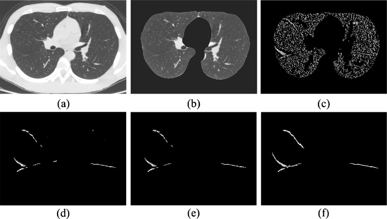
Our method consists of five steps, including lung segmentation, plane-like structure enhancement, surface extraction with LBD, initial fissure identification with MBI, and fissure extension based on local plane fitting (Fig. 1).
Fig. 1.
2D figures of the segmented fissures in different stages. a Original image, b lung segmentation image, c plane enhancement image, d surfaces extracted with LBD, e initial fissures identified with MBI, and f final fissure determined by local plane fitting based on initial fissures
Lung Segmentation
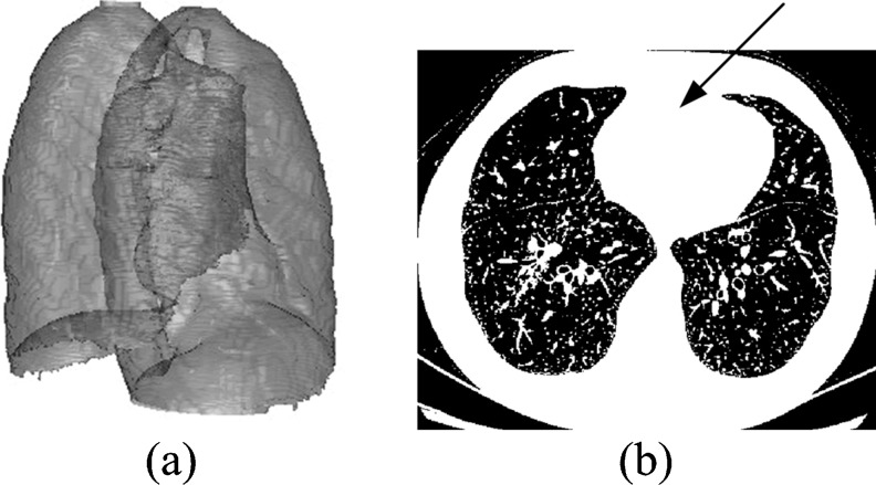
For the purpose of reducing the influence of other tissues outside the lung regions, lung segmentation is performed and its result is shown in Fig. 2. Successive steps of the approach are performed inside the segmented lung areas.
Fig. 2.
The segmented results of the lung area: a 3D surface rendering of the segmented lungs and b the threshold results, with a black arrow pointing to the biggest connected area
The method of lung segmentation is described as follows:
Based on the histogram of the volume images in the range of CT values, a suitable threshold is selected by Otsu’s method [10] for converting the images into the binary images. Zero is set to the voxels with CT values lower than the threshold, while 1 is set to the others (Fig. 2b). The 0 areas cover the air inside the lung and trachea and outside the body, while the 1 areas cover the body tissues and the bed.
As pointed by the black arrow in Fig. 2b, the biggest 26-connected volume of voxels with a value of 1 is found and regarded as the body area, and then the 0 regions enclosed in the body area are regarded as the lung areas. Now, the lung areas are roughly obtained with some segmentation offsets caused by the irregular pleurae and tracheas.
The morphologic rolling ball technique [11] is applied to smooth the irregular pleurae and the boundary identification bridge method [12] is used to enclose the trachea regions within the lung area. Then, we obtain the complete lung areas and their corresponding 3D contours, denoted as Sc, as shown in the Fig. 2a.
Plane-Like Structure Enhancement with the Hessian Matrix
Once the lung areas were identified, a plane enhancement filter is applied to detect planar structures. The enhancement filters based on the Hessian matrix can be used to detect dot-like nodules, line-like vessels, and plane-like tissues [13]. However, the detection effect is sensitive to noises, so the CT images should be smoothed with a 3D Gaussian template. For better smooth performance, the scale parameter σ of the 3D Gaussian template should be chosen as large as possible, but it cannot be larger than half of the thickness of the fissures. Thus, the scale σ is considered as 1 voxel width.
Let f(x, y, z) be the CT value of the voxel (x, y, z) in the smoothed CT image. Then, the eigenvalues λ0(x, y, z), λ1(x, y, z), and λ2(x, y, z) (|λ0(x, y, z)| ≥ |λ1(x, y, z)| ≥ |λ2(x, y, z)|) and their corresponding unit eigenvectors v0(x, y, z), v1(x, y, z), and v2(x, y, z) of the Hessian matrix are calculated for each voxel inside the lung areas. For an ideal brighter plane, an ideal brighter line, and an ideal brighter dot, three eigenvalues must satisfy, respectively [12]:
 |
1 |
 |
2 |
 |
3 |
Due to the CT values of fissures ranging between −800 and −400 Hounsfield units (HU) [5], the plane-like structure enhancement function is defined as:
 |
4 |
Figure 1c shows the enhancement results of the plane-like structures based on the Hessian matrix.
Surface Extraction with LBD
Now that voxels on the fissures besides some other plane-like structures have been enhanced, we remove the voxels on the lung borders based on the previous lung segmentation results and use an empirical threshold T1 to delete the voxels with weak plane enhancement. So, the set of the remaining voxels Se is defined as:
 |
5 |
Empirically, T1 = 0.3 was selected to settle the trade-off between suppressing the non-plane structures and keeping the lower contrast thin fissures. But due to the similar enhancement of the voxels on the fissures and the walls of other tissues, many non-fissure voxels are still left. So, we propose to define the LBD based on the eigenvectors of the Hessian matrix to refine the selected surfaces.
For a voxel (x, y, z) on the plane-like structures, the eigenvector v0(x, y, z) corresponding to the largest absolute value of eigenvalue λ0(x, y, z) represents the direction of the biggest CT value change, which is orthogonal to the local plane centered at the voxel (x, y, z). Thus, v0(x, y, z) is the normal vector of this local plane, and the included angle between two local planes of the neighboring voxels can be described by the included angle between their normal vectors. If these two planes belong to the same flat surface, their normal vectors are approximately parallel. On the contrary, if they belong to the different flat surfaces, their normal vectors have an included angle. Thus, the LBD between two 26-adjacent voxels u and w, denoted by LBD(u, w), is given by the cosine of the included angle between their corresponding local planes, i.e., the inner product of the normal vectors. Noticing that the cosine function is decreasing in [0, π], we define the LBD as follow:
 |
6 |
Then, each group of the connected voxels is extracted as a candidate surface using the 3D region-growing method under the constraints of LBD. We describe the candidate surface extraction algorithm as follows.
Algorithm surface extraction
During the region-growing procedure, constraints on the LBD limit the local shape of the surfaces. Furthermore, the fissures should commonly appear as large connected regions. So, if the number of voxels in a connected surface is smaller than an empirical threshold T2 = 200, it will be discarded. Figure 1d shows the extracted surfaces, where many small surfaces and surfaces having large LBD are eliminated. The extracted surfaces no longer need to be smoothed because the Hessian matrix is calculated based on the smoothed image. Owing to the low contrast of voxels or sudden change in shape, the fissures might be broken into isolate patches and/or there might be some holes left on it. The remaining surfaces will be remedied in the follow-up steps.
Initial Fissure Identification with MBI
After the previously described steps, the remaining connected surfaces are the larger ones with less bending deformation in some direction, mainly containing the fissures and the walls of other tissues such as vessels and bronchi. Nevertheless, the fissures are planar objects and the walls of vessels and bronchi are cylindrical ones.
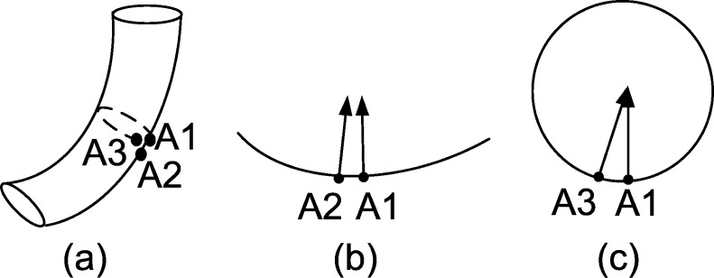
As shown in Fig. 3, the bending degree of the cylinder-like surface differs significantly in different directions. Generally, the bending degree along the axial direction of the cylindrical surfaces is the smallest; on the other hand, the bending degree perpendicular to the axial direction is large and its quantity depends on the diameter of the cylinder.
Fig. 3.
Comparison of two curvatures in different directions of the cylindrical surface: a the cylindrical surface, with A1 adjacent to A2 and A3, respectively, in the cross and lateral sections, b the lateral section, and c the cross section
In Fig. 3, a cylinder model (Fig. 3a) for simulating the walls of the cylinder-like tissues, with its lateral section (Fig. 3b) and cross section (Fig. 3c), is shown. A1 adjoins A2 and A3, respectively, at two different directions. Orientation of the arrow depicts the normal vector direction of the local surface at the current point. As we can see, even though the included angle between the vectors centered at A1 and A2 is small, the direction change of the vectors centered at A1 and A3 is still significant.
In real CT chest images, the diameters of the blood vessels and bronchi are smaller than 15 mm, so the bending degree perpendicular to the axial is much bigger than the one along the axial. However, the bending degree along all directions in the planar surface is basically similar.
Therefore, to effectively distinguish cylinder surfaces from planes, we propose to define the MBI of the surfaces. The MBI of the i-th surface, denoted by MBI(i), is defined as:
 |
7 |
where S(i) is the set of voxels belonging to the i-th surface. We set the mean MBI of all surfaces as a threshold to delete the cylinder surfaces. Thus, in the remaining surfaces, the ones containing more than 5,000 voxels are regarded as the initial fissures (Fig. 1e) and the others are regarded as the isolate plane patches.
Fissure Extension by Using Local Plane Fitting
In the previous steps, for avoiding misdetection, some uncertain fissure patches are neglected by making stricter fissure segmentation criteria (i.e., the restrictions on the LBD, the MBI, and the surface size). As a consequence, the missing fissure patches should be retrieved to mend those strictly determined initial fissures. Because the adjacent patches of the fissures orientate basically the same, the discontinue patches can be mended to form the complete fissures based on the local plane fitting.
First, the local plane fitting is used to fill the holes in the initial fissures and the gaps between the initial fissures and the isolate plane patches. We employ a 3D window with the size of 15 × 15 × 15 moving across the grid in step length of 1 voxel in each of three directions, respectively. The size of the window is determined empirically. If the size is too big, computation takes a long time; if the size is too small, there are many windows with less than 4 voxels where the plane fitting method is inapplicable. At each position of the window, if at least 3 voxels besides the window center belong to the initial fissures, we can construct a fitting plane which can be formulated by the following equation:
 |
8 |
where a, b, c, and d are the coefficients of the fitting plane determined by the modified Golub–Reinsch algorithm [14]. Once the plane equation is determined, Eq. 8 is used to find all voxels on the plane and in the window and to add them into the fissures.
Then, all voxels in one isolate plane patch can be added into the fissures, if there exist a voxel in this patch and a voxel in the existing extended fissures, which are 26-connected neighbors of each other and the LBD between them is less than 0.5.
Evaluation
Because the reference segmentation is delineated slice by slice, we apply a 2D evaluation rather than the 3D ones to assess the performance of our segmentation approach.
The positive predictive value (PPV) is used to quantify how consistent are the segmented results with the reference standard. It is defined as the proportion of the number of correctly segmented voxels to the total number of voxels in the segmented fissures. Here, the correctly segmented voxels include all the segmented voxels which are less than 2 mm away from the closest voxel of the reference standard in the same slice, i.e.:
 |
9 |
where Sseg is the set of the fissure voxels segmented automatically by our approach, Sref is the set of the fissure voxels provided manually as the gold standard, and D2(•) means the 2D Euclidean distance of 2 voxels in the same slice.
Sensitivity (SENS) is also applied to provide information on whether the segmented results are actually included in the reference fissures.
 |
10 |
An exact segmentation will have a high PPV and a high SENS. However, PPV and SENS do not reveal how far the distance is between the results and the reference fissures. Thus, we use two distance measures as complementary criteria, including the root–mean square (RMS) distance and its standard deviation. RMS was defined as [5]:
 |
11 |
where D3(•) represents the 3D Euclidean distance of 2 voxels. The mean RMS indicates the positioning accuracy of the approach. The standard deviation implies the stability of the algorithm and the maximal RMS represents the maximal error.
Results
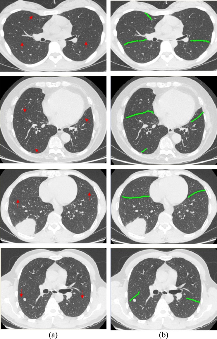
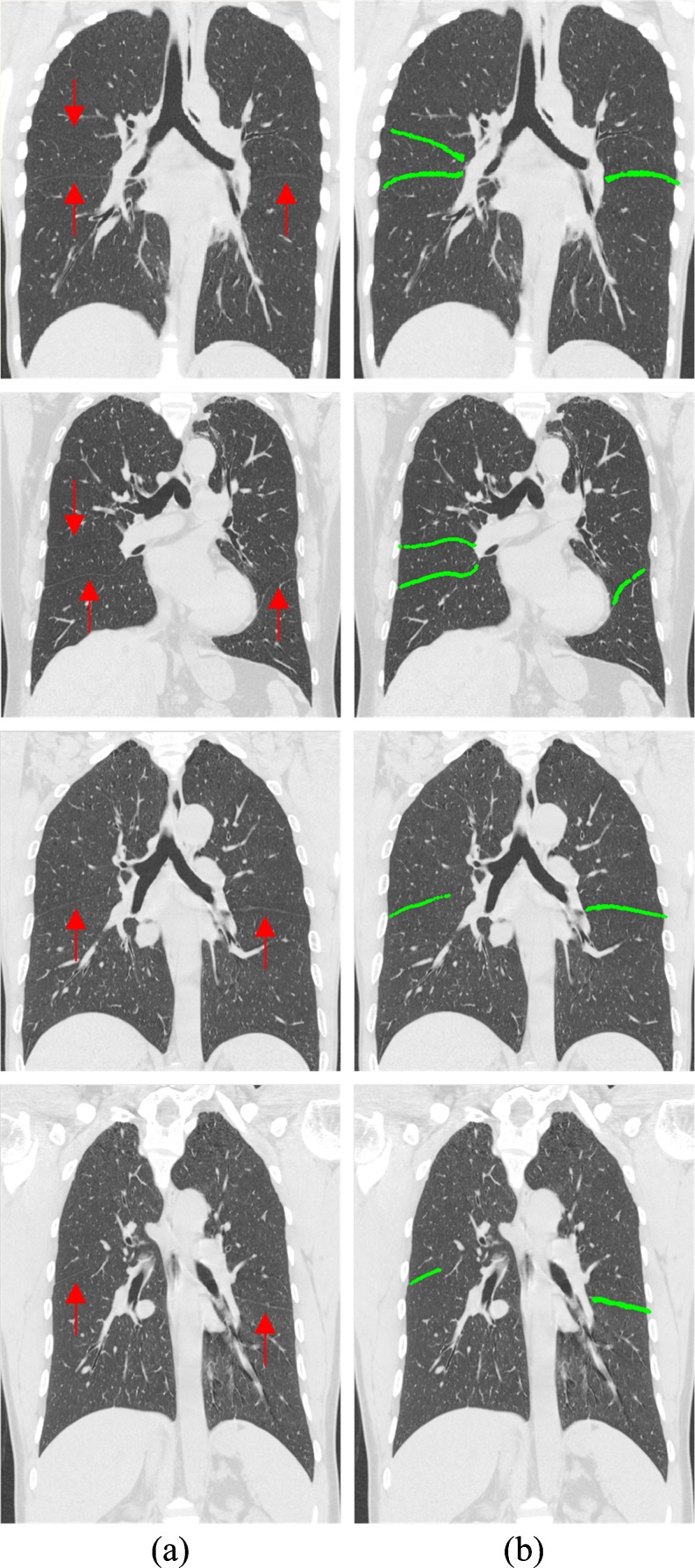
Figures 4, 5, and 6 illustrate the results of some fissures segmented by our approach of the axial views, sagittal views, and coronal views, respectively. Each row corresponds to an axial CT image of the case. The original CT images and the segmentation results marked in green are shown in each column. As shown in Figs. 4a, 5a, and 6a, where the fissures are indicated by red arrows, the locations, shapes, and sizes of the fissures vary greatly from case to case. However, the results of the proposed method follow the fissures very well. As we can see in Figs. 4b, 5b, and 6b, both the oblique and horizontal fissures are relatively complete. Table 1 lists the PPV, SENS, mean RMS distance, and maximal RMS distance for our segmentation technique, ranging from 87 %, 80 %, 0.81 mm, and 7.98 mm to 96 %, 94 %, 1.35 mm, and 15.2 mm, respectively. And the means of the PPV, SENS, RMS distance, and maximal RMS distance of 15 cases are 91 %, 88 %, 1.02 ± 1.00 mm, and 11.56 mm, respectively. It shows that the segmented fissures follow the reference fissures well, but still a few fissure voxels with CT values similar to their surroundings are missing, and a few non-fissure voxels similar to fissure voxels’ CT values and very close to the fissures are falsely included.
Fig. 4.
Some fissure segmentation results produced by our proposed method with the reference standard. a Original image in axial view where the fissures were indicated by the red arrows and b segmentation results marked in green
Fig. 5.
Some fissure segmentation results produced by our proposed method with the reference standard. a Original image in sagittal view where the fissures were indicated by the red arrows and b segmentation results marked in green
Fig. 6.
Some fissure segmentation results produced by our proposed method with the reference standard. a Original image in coronal view where the fissures were indicated by the red arrows and b segmentation results marked in green
Table 1.
Performance of our segmentation method, including PPV, SENS, RMS distances, and maximal RMS distances of 15 chest CT scans
| Case | PPV (%) | SENS (%) | RMS (mm) | Maximal RMS (mm) |
|---|---|---|---|---|
| 1 | 95 | 93 | 0.95 ± 0.73 | 11.71 |
| 2 | 88 | 90 | 1.07 ± 0.94 | 11.46 |
| 3 | 92 | 86 | 0.93 ± 1 | 12.76 |
| 4 | 93 | 90 | 0.85 ± 1.01 | 14.16 |
| 5 | 92 | 80 | 0.97 ± 1.01 | 11.53 |
| 6 | 96 | 94 | 0.81 ± 0.65 | 9.2 |
| 7 | 94 | 88 | 0.89 ± 0.64 | 8.92 |
| 8 | 92 | 86 | 0.95 ± 0.84 | 11.06 |
| 9 | 89 | 89 | 1.04 ± 1.11 | 11.46 |
| 10 | 89 | 84 | 1.16 ± 1.23 | 11.16 |
| 11 | 88 | 83 | 1.12 ± 1.27 | 13.54 |
| 12 | 87 | 94 | 1.11 ± 1.08 | 12.88 |
| 13 | 89 | 85 | 0.99 ± 0.8 | 7.98 |
| 14 | 88 | 91 | 1.35 ± 1.52 | 15.2 |
| 15 | 88 | 91 | 1.12 ± 1.1 | 10.34 |
| Average | 91 | 88 | 1.02 ± 1.00 | 11.56 |
Discussion
Our main contributions include three aspects. First, we propose the LBD to measure the local flatness of the surface. Then, the region-growing algorithm based on the LBD is applied to extract candidate surfaces. As a result, the surfaces with complex local shapes are discarded. The isolate small structures are eliminated by using an empirical threshold for sizes of the surface. Second, we apply the MBI to identify the initial fissures and isolate plane patches, which can effectively distinguish the fissures from the walls of cylinder-like tissues such as vessels and bronchi. Third, the local plane fitting is used to extend fissures to fill the holes in the fissures and connect the isolate patches.
In our approach, the eigenvalues of the Hessian matrix are used to enhance the plane-like structures, which have also been utilized by van Rikxoort et al. [6, 8] and Wiemker et al. [7]. But in Wiemker et al. [7] and van Rikxoort et al. [8], the quantitative performance of fissure segmentation was not reported and the walls of other tissues were still left because only the eigenvalues and no eigenvectors of the Hessian matrix were used. Then, in van Rikxoort et al. [6], a supervised enhancement filter was applied to improve the performance of Wiemker et al. [7] and van Rikxoort et al. [8]; in their method, manual segmentation was required to train the system and the whole process, including training and testing, would spend more time. Rather than take an extra training process, our system directly exploits the LBD, that is, the cosine of the included angle between the eigenvectors of two Hessian matrices for a pair of adjacent voxels, and the MBI, so that it is more convenient to be implemented. We propose to apply the eigenvectors of the Hessian matrix, so the walls of other tissues can be effectively distinguished from the fissures.
For the differences in data obtaining and processing, we could not directly compare our results with other literatures. However, in the existing publications on fissures segmentation, Wang et al. [3], Zhang et al. [4], and Pu et al. [5] had reported RMS distances as the quantitative analysis of the performance. The method of Wang et al. [3] had been applied to 10 cases, and their mean RMS was 1.38 ± 1.01 mm. Tested on 22 cases, the technique of Zhang et al. [4] acquired the mean RMS distance of 1.96 ± 0.71 mm. The results of Pu et al. [5] were obtained with 100 images from 10 cases, and their RMS distances ranged from 1.48 ± 0.92 to 2.04 ± 3.88 mm. It is obvious that the RMS of our approach is lower than their results, so that the fissures segmented by our approach are closer to the true fissures.
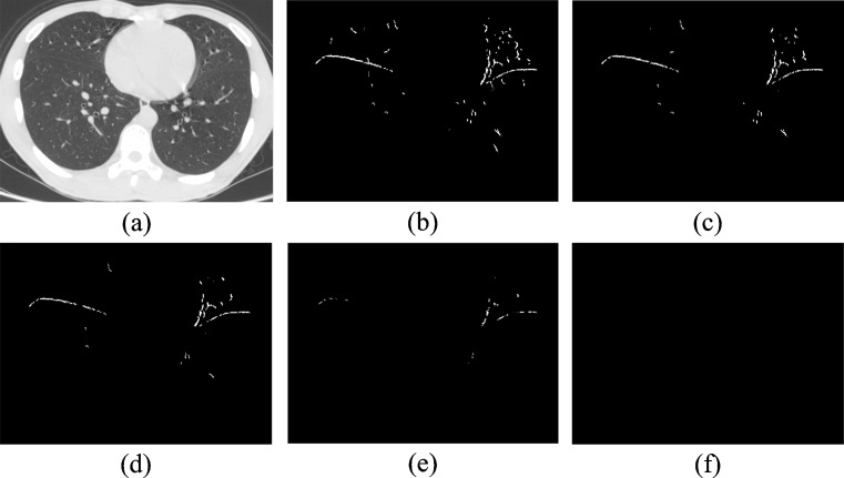
Two parameters, T1 and T2, have impacts on surface identification, which are selected by observing the results of two cases with different parameters. Figure 7 shows five different results by assigning five different values to T1, ranging from 0.1 to 0.9, and assigning 200 to T2. While T1 is increasing, fewer surfaces are extracted and the holes in the surfaces and the gaps between surfaces are getting bigger so that they are hard to be filled in the fissure extension step. When T1 is equal to or bigger than 0.7, lots of major fissures are missing, whereas, when T1 is smaller than 0.3, many false planes stuck to the major fissures are left, which are hard to be eliminated in the later steps. T1 in the range between 0.3 and 0.7 ensures to keep most plane structures and also to suppress most non-plane structures. But we found that, when T1 is bigger than 0.3, holes differ enormously in size, which increases the difficulty of filling holes. Thus, we set T1 equal to 0.3.
Fig. 7.
Surface extraction with T 2 = 200 and different T 1 values: a original image, b T 1 = 0.1, c T 1 = 0.3, d T 1 = 0.5, e T 1 = 0.7, and d T 1 = 0.9
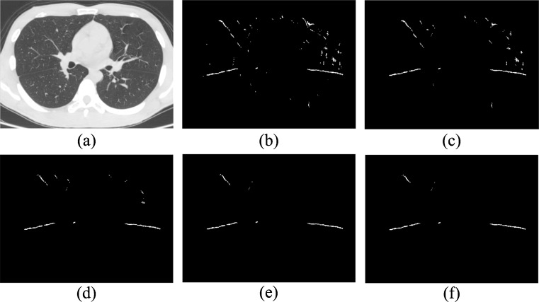
The appropriate T2 is used to eliminate the small plane surfaces dominated by non-fissure planes. Figure 8 shows five different results by assigning T1 = 0.3 and assigning six different values to T2, ranging from 50 to 400. When T2 is smaller than 200, more surfaces are extracted and non-fissure surfaces increase dramatically. With increasing of T2, the number of non-fissure surfaces, as well as fissure surfaces, decreases. Especially when T2 is bigger than 300, there are too many missing fissure patches to be filled in the extension step. With T2 in the range between 200 and 300, the number of extracted surfaces has stabilized and most fissure surfaces can be left. Thus, to minimize the missing fissure surfaces and stabilize the results, we set T2 equal to 200. So far, the tested samples are high-dose examinations; future work is aimed at applying the proposed method on low-dose examinations.
Fig. 8.
Surface extraction with T 1 = 0.3 and different T 2 values: a original image, b T 2 = 50, c T 2 = 100, d T 2 = 200, e T 2 = 300, and d T 2 = 400
Conclusion
We have developed an automatic training-free segmentation approach of pulmonary fissures in CT images. Based on the 3D geometric morphology knowledge of fissures, we propose the concepts of LBD and MBI. The LBD represents the local surface flatness in 3D space. Due to the walls of non-fissure structures having a similar local feature to the fissures, the MBI is defined to distinguish cylindrical surfaces and planes in order to suppress non-fissure structures. In the end, local plane fitting is used to fill the holes of fissures and connect the isolate patches of fissures. Our approach achieves a better performance compared with the existing training-free systems and achieves basically the same performance compared with the existing training-required methods, but our method does not need a training process.
References
- 1.Gulsun M, Ariyurek OM, Comert RB, Karabulut N. Variability of the pulmonary oblique fissures presented by high-resolution computed tomography. Surg Radiol Anat. 2006;28:293–299. doi: 10.1007/s00276-006-0079-y. [DOI] [PubMed] [Google Scholar]
- 2.Kubo M, Niki N, Nakagawa S, Eguchi K, Kaneko M, Moriyama N, Omatsu H, Kakinuma R, Yamaguchi N. Extraction algorithm of pulmonary fissures from thin-section CT images based on linear feature detector method. IEEE Trans Nucl Sci. 1999;46:2128–2133. doi: 10.1109/23.819294. [DOI] [Google Scholar]
- 3.Wang JB, Betke M, Ko JP. Pulmonary fissure segmentation on CT. Med Image Anal. 2006;10:530–547. doi: 10.1016/j.media.2006.05.003. [DOI] [PMC free article] [PubMed] [Google Scholar]
- 4.Zhang L, Hoffman EA, Reinhardt JM. Atlas-driven lung lobe segmentation in volumetric X-ray CT images. IEEE Trans Med Imaging. 2006;25:1–16. doi: 10.1109/TMI.2005.859209. [DOI] [PubMed] [Google Scholar]
- 5.Pu JT, Leader JK, Zheng B, Knollmann F, Fuhrman C, Sciurba FC, Gur D. A computational geometry approach to automated pulmonary fissure segmentation in CT examinations. IEEE Trans Med Imaging. 2009;28:710–719. doi: 10.1109/TMI.2008.2010441. [DOI] [PMC free article] [PubMed] [Google Scholar]
- 6.van Rikxoort EM, van Ginneken B, Klik M, Prokop M. Supervised enhancement filters: Application to fissure detection in chest CT scans. IEEE Trans Med Imaging. 2008;27:1–10. doi: 10.1109/TMI.2007.900447. [DOI] [PubMed] [Google Scholar]
- 7.Wiemker R, Bulow T, Blaffert T: Unsupervised extraction of the pulmonary interlobar fissures from high resolution thoracic CT data. International Congress Series 1281:1121–1126, 2005
- 8.van Rikxoort EM, Prokop M, de Hoop B, Viergever MA, Pluim J, van Ginneken B. Automatic segmentation of pulmonary lobes robust against incomplete fissures. IEEE Trans Med Imaging. 2010;29:1286–1296. doi: 10.1109/TMI.2010.2044799. [DOI] [PubMed] [Google Scholar]
- 9.Gu S, Wilson D, Wang Z, Bigbee WL, Siegfried J, Gur D, Pu J. Identification of pulmonary fissures using a piecewise plane fitting algorithm. Comput Med Imaging Graph. 2012;36:560–571. doi: 10.1016/j.compmedimag.2012.06.001. [DOI] [PMC free article] [PubMed] [Google Scholar]
- 10.Otsu N. A threshold selection method from gray-level. IEEE Trans Syst Man Cybern SMC. 1979;9:62–66. doi: 10.1109/TSMC.1979.4310076. [DOI] [Google Scholar]
- 11.Silva AC, Carvalho PCP, Nunes R, et al: Segmentation and reconstruction of the pulmonary parenchyma. Vision and Graphics Laboratory, Institute of Pure and Applied Mathematics, Rio de Janeiro, 2002, pp 1–12
- 12.Armato SG, Giger ML, Moran CJ, Blackburn JT, Doi K, MacMahon H. Computerized detection of pulmonary nodules on CT scans. Radiographics. 1999;19:1303–1311. doi: 10.1148/radiographics.19.5.g99se181303. [DOI] [PubMed] [Google Scholar]
- 13.Li Q, Sone S, Doi K. Selective enhancement filters for nodules, vessels, and airway walls in two- and three-dimensional CT scans. Med Phys. 2003;30:2040–2051. doi: 10.1118/1.1581411. [DOI] [PubMed] [Google Scholar]
- 14.Chan TF. An improved algorithm for computing the singular value decomposition. ACM Trans Math Softw. 1982;8(1):72–83. doi: 10.1145/355984.355990. [DOI] [Google Scholar]


