Abstract
It is difficult for radiologists to classify pneumoconiosis from category 0 to category 3 on chest radiographs. Therefore, we have developed a computer-aided diagnosis (CAD) system based on a three-stage artificial neural network (ANN) method for classification based on four texture features. The image database consists of 36 chest radiographs classified as category 0 to category 3. Regions of interest (ROIs) with a matrix size of 32 × 32 were selected from chest radiographs. We obtained a gray-level histogram, histogram of gray-level difference, gray-level run-length matrix (GLRLM) feature image, and gray-level co-occurrence matrix (GLCOM) feature image in each ROI. For ROI-based classification, the first ANN was trained with each texture feature. Next, the second ANN was trained with output patterns obtained from the first ANN. Finally, we obtained a case-based classification for distinguishing among four categories with the third ANN method. We determined the performance of the third ANN by receiver operating characteristic (ROC) analysis. The areas under the ROC curve (AUC) of the highest category (severe pneumoconiosis) case and the lowest category (early pneumoconiosis) case were 0.89 ± 0.09 and 0.84 ± 0.12, respectively. The three-stage ANN with four texture features showed the highest performance for classification among the four categories. Our CAD system would be useful for assisting radiologists in classification of pneumoconiosis from category 0 to category 3.
Keywords: Computer-aided diagnosis (CAD), Chest radiography, Artificial neural network, Pneumoconiosis, Texture feature
Introduction
Workers in the shipbuilding and metal goods manufacturing industry who inhale silica and/or coal dust are at an increased risk of developing pneumoconiosis. Therefore, they routinely undergo lung function tests and chest radiography. Specifically, according to the guidelines of the International Labor Organization (ILO) and the Ministry of Labor, Japan, radiologists subjectively classify radiolucencies on standard chest radiographs according to profusion, shape, and size [1–3]. Category 0 (normal case) refers to the absence of small opacities or the presence of small opacities that are less profuse than those in category 1 [2]. Profusion is determined by comparison with standard radiographs and recorded as one of the following categories: 0, 1, 2, or 3 [2]. However, it is difficult for radiologists to classify pneumoconiosis with small and irregular opacities [4]. Therefore, a number of researchers have developed computer-aided diagnosis (CAD) schemes for detecting pneumoconiosis on chest radiographs to assist radiologists as a “second opinion” in image interpretation.
Such CAD systems for detection of interstitial lung disease and pneumoconiosis on chest radiographs apply root mean square (RMS) variation, texture analysis based on the Fourier transform, geometric pattern feature analysis methods, and artificial neural network (ANN) methods [5–17]. Yu et al. segmented the lung field with pneumoconiosis using feature extraction based on the multi-scale difference filtering histogram and the gray-level co-occurrence matrix (GLCOM) [15]. Zhu et al. segmented the lung field using the combining Otsu’s threshold method with morphological reconstruction followed by subdivision into six regions [16]. They developed a computerized scheme for classification between normal and abnormal regions with 22 wavelet-based energy texture features and a support vector machine (SVM) [16].
CAD systems for detection of diffuse lung disease on computed tomography (CT) images applied a gray-level run-length matrix (GLRLM), GLCOM, and a multi-scale filter bank [18–21]. Uchiyama et al. attempted to determine six physical measures with the mean and standard deviation of the CT value, air density components, nodular components, line components, and multi-locular components [20]. Wang et al. developed an automated method with new texture features determined from GLRLM [21].
Many researchers have applied the ANN in classification of normal and abnormal or malignant and benign lesions on chest radiographs and CT images [22–26]. In addition, the ANN has been applied in differential diagnosis of interstitial lung diseases on chest radiographs [27] and CT images [28], hepatic masses on CT images [29], and hepatic fibrosis on magnetic resonance (MR) images [30]. Ashizawa et al. selected 11 interstitial lung diseases based on 10 clinical parameters (age, sex, duration of symptoms, temperature, etc.) and 16 radiological findings (distribution of infiltrates, characteristics of infiltrates, etc.) extracted by chest radiologists [27]. Fukushima et al. selected 10 clinical parameters and 23 CT features (extent of lesion, distribution of lesion, characteristics of lesion, nodular opacity, decreased lung opacity, etc.) extracted on chest CT images [28]. They developed the ANN for the differential diagnosis of 11 diffuse lung diseases (sarcoidosis, diffuse panbronchiolitis, non-specific interstitial pneumonia, lymphangitic carcinomatosis, interstitial pneumonia, etc.) on chest radiographs and CT images [27, 28].
For classification of two cases, such as normal vs. abnormal or malignant vs. benign lesions, ANN consisted of a number of input units and one output unit. We developed a CAD system to distinguish between normal (category 0) and abnormal (category 1, 2, or 3) regions of interest (ROIs) in pneumoconiosis using the ANN trained with the power spectrum (PS) values [31]. In addition, we developed a rule-based plus ANN method to distinguish between normal and abnormal ROIs using the window function, top-hat transformation, and GLCOM analysis [32]. The areas under the receiver operating characteristic (ROC) curves for category 3 (severe pneumoconiosis) and category 1 (early pneumoconiosis) were 0.93 ± 0.02 and 0.72 ± 0.03, respectively [32].
Many groups have reported computerized schemes for higher classification between normal and abnormal regions on chest radiographs and CT images. However, because the diagnosis influences the recognition of the workers’ handicap, it is necessary for the radiologist to correctly classify pneumoconiosis from category 1 (early pneumoconiosis) to category 3 (severe pneumoconiosis). In addition, ANNs have been useful for classification of a number of cases, such as the differential diagnosis of interstitial lung, hepatic masses, and hepatic fibrosis [27–30]. There have been no studies regarding the classification performance among four categories of pneumoconiosis with ANN. Therefore, we have developed a new CAD system based on a three-stage ANN with four texture features for case-based classification among four categories of pneumoconiosis on chest radiographs. We also investigated the effects of ROI-based classification with various parameters on four texture features with the first ANN.
Materials and Methods
Materials
As shown in Table 1, we used 38 posteroanterior (PA) chest radiographs developed by the Ministry of Labor. These included three normal cases, five cases of silicosis (category 1: three cases, category 2: one case, category 3: one case), five cases of asbestosis (category 1: two cases, category 2: two cases, category 3: one case), six cases of other pneumoconiosis (category 1: four cases, category 2: one case, category 3: one case), four cases of category 0 (normal case), six cases of category 1, six cases of category 2, and three cases of category 3 with pneumoconiosis [3, 33]. In addition, we used 17 PA chest radiographs developed by ILO. These included two cases of category 0 (normal case), five cases of category 1, five cases of category 2, and five cases of category 3 with pneumoconiosis [2]. The small opacities were classified into four categories, ranging from a completely normal case (category 0) to severe pneumoconiosis (category 3) [2]. These images were digitized with a pixel size of 0.175 mm, matrix sizes of 2468 × 2034 and 2034 × 2034, and 12-bit gray level.
Table 1.
Number of cases in the digital image database developed by the Ministry of Labor and ILO
| Name of digital image database | Category 0 | Category 1 | Category 2 | Category 3 |
|---|---|---|---|---|
| The Ministry of Labor | 7 cases | 15 cases | 10 cases | 6 cases |
| The International Labor Organization | 2 cases | 5 cases | 5 cases | 5 cases |
| Total number of cases | 9 cases | 20 cases | 15 cases | 11 cases |
Overall Scheme of Pneumoconiosis Classification with Four Categories
Figure 1 shows the overall scheme of the classification with four texture features. An experienced radiological technologist manually selected approximately 100–1200 ROIs on the lung with a matrix size of 32 × 32 in the intercostal spaces and over rib spaces for each chest radiograph [5]. We eliminated overlap with ROIs. Table 2 shows the number of ROIs selected for each case. We obtained a background trend in all selected ROIs using a two-dimensional surface-fitting technique based on the least squares method [5]. After the number of gray levels in these ROIs was reduced by quantization level, we then obtained gray-level histograms, histograms of gray-level differences, GLRLM feature images, and GLCOM feature images. The first ANN was trained with each texture feature for the ROI-based classification of patterns among the four categories. Next, the second ANN was trained with combined patterns including output values obtained from the first ANN with each texture feature. Finally, we obtained the case-based classification performed for distinguishing among the four categories with the third ANN.
Fig. 1.
Architecture of the computerized classification method using three-stage ANN
Table 2.
Number of ROIs per case defined as category 0 to category 3
| The Ministry of Labor | |||
| Number of ROIs | |||
| Category | No. of cases | Abnormal ROI | Normal ROI |
| Category 0 | No. 1 | 0 | 48 |
| No. 2 | 0 | 75 | |
| No. 3 | 0 | 47 | |
| No. 4 | 0 | 99 | |
| No. 5 | 0 | 128 | |
| No. 6 | 0 | 98 | |
| No. 7 | 0 | 19 | |
| Category 1 | No. 1 | 6 | 90 |
| No. 2 | 17 | 141 | |
| No. 3 | 135 | 40 | |
| No. 4 | 21 | 44 | |
| No. 5 | 113 | 50 | |
| No. 6 | 207 | 40 | |
| No. 7 | 202 | 44 | |
| No. 8 | 218 | 36 | |
| No. 9 | 244 | 23 | |
| No. 10 | 242 | 3 | |
| No. 11 | 138 | 30 | |
| No. 12 | 478 | 4 | |
| No. 13 | 312 | 0 | |
| No. 14 | 418 | 104 | |
| No. 15 | 77 | 23 | |
| Category 2 | No. 1 | 303 | 24 |
| No. 2 | 333 | 20 | |
| No. 3 | 169 | 39 | |
| No. 4 | 416 | 18 | |
| No. 5 | 713 | 0 | |
| No. 6 | 1175 | 0 | |
| No. 7 | 353 | 53 | |
| No. 8 | 300 | 0 | |
| No. 9 | 153 | 0 | |
| No. 10 | 162 | 0 | |
| Category 3 | No. 1 | 475 | 0 |
| No. 2 | 213 | 43 | |
| No. 3 | 330 | 34 | |
| No. 4 | 895 | 0 | |
| No. 5 | 332 | 0 | |
| No. 6 | 1266 | 0 | |
| The International Labor Organization | |||
| Number of ROIs | |||
| Category | No. of cases | Abnormal ROI | Normal ROI |
| Category 0 | No. 1 | 0 | 101 |
| No. 2 | 0 | 96 | |
| Category 1 | No. 1 | 240 | 21 |
| No. 2 | 324 | 22 | |
| No. 3 | 96 | 33 | |
| No. 4 | 255 | 30 | |
| No. 5 | 31 | 96 | |
| Category 2 | No. 1 | 302 | 61 |
| No. 2 | 346 | 0 | |
| No. 3 | 316 | 27 | |
| No. 4 | 215 | 14 | |
| No. 5 | 219 | 16 | |
| Category 3 | No. 1 | 356 | 23 |
| No. 2 | 341 | 24 | |
| No. 3 | 481 | 0 | |
| No. 4 | 495 | 0 | |
| No. 5 | 289 | 0 | |
Four Texture Features
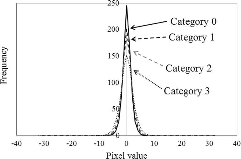
First, the gray-level histogram was applied to the trend-corrected images quantized to the 4-bit gray level. Compared with the images in category 3, the frequencies of pixel values 6 and 7 were higher for the images in the other categories (Fig. 2). The histogram of gray-level differences indicated the frequency of the difference of gray levels i and j at a specified distance d and specified direction θ. The histogram of the gray-level difference (distance level: 7 pixels and direction: 0°) was applied to the trend-corrected images quantized to the 5-bit gray level. Compared with category 3, the frequencies of the other categories were higher in the 0-pixel value (Fig. 3). The effects of the number of gray levels and the distance levels on the gray-level histograms and histograms of gray-level differences in the ROI-based classification among the four categories will be discussed later.
Fig. 2.
Gray-level histograms from four categories on 4-bit gray level
Fig. 3.
Histograms of gray-level differences from four categories on 5-bit gray level
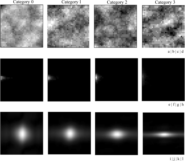
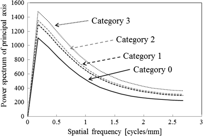
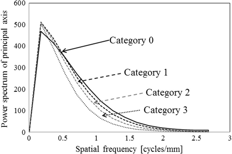
A gray-level run-length was defined as a set of consecutive pixels of the same gray level in a given direction [21]. An element of a GLRLM measures the number of occurrences of a run with a specific gray level in a given direction [21]. In this study, the GLRLM feature images (direction: 0°) were applied to the trend-corrected images quantized to the 6-bit gray level (Fig. 4e–h). The horizontal and vertical directions of the GLRLM feature images were composed of the length of runs and the number of gray levels, respectively (Fig. 4e–h). These four categories showed quite different values in some parts of the GLRLM feature images. For example, as the profusion of small opacities was concentrated from category 0 to category 3, the GLRLM feature images for category 0 showed many long runs at the lower pixel values (Fig. 4e), whereas the GLRLM feature images for category 3 showed many short runs at the highest pixel values (Fig. 4h). We then determined the power spectrum (PS) images in these GLRLM feature images by fast Fourier transform (Fig. 4i–l). We used only PS values on the principal and secondary axes, which represent the maximum and next maximum PS values on the radial line from the central point, respectively [31, 32]. We used the PS values on the positive main and second axes representing spatial frequency, because they were symmetric with respect to the center of the PS image (Fig. 5) [31, 32]. Compared with category 3, the PS values of the other categories were lower at all spatial frequencies on the principal and secondary axes. The effects of the number of gray levels on the GLRLM feature images on the ROI-based classification among the four categories will be discussed later.
Fig. 4.
GLRLM feature image and PS obtained by Fourier transform of the GLRLM feature images for four categories (a–d). Trend-corrected images among the four categories (e–h). GLRLM feature images among the four categories (i–l). PS images of the GLRLM feature images among the four categories
Fig. 5.
PS values on the principal axis of the GLRLM feature image
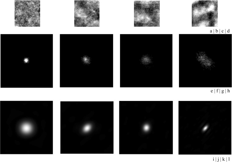
An element at location (i, j) of the GLCOM showed that the joint probability density function indicated the possibility of gray level between the i pixel and the j pixel in a specified direction θ and a specified distance d [15]. In the same manner as for the GLRLM feature images, the GLCOM feature images (distance level: 3 pixels and direction: 45°, 225°) were applied to the trend-corrected images quantized to the 6-bit gray level (Fig. 6e–h). The horizontal and vertical directions of the GLCOM feature images were composed of the number of gray levels [32]. We calculated PS images by Fourier transform (Fig. 6i–l) and obtained only the PS values on the principal and secondary axes (Fig. 7) [32]. The PS values for each category were different at spatial frequencies of 0.5–1.5 on the principal and secondary axes. The effects of the distance levels on the GLCOM feature images on ROI-based classification among the four categories will be discussed later.
Fig. 6.
GLCOM feature images and PS obtained by Fourier transform of the GLCOM feature images for the four categories (a–d). Trend-corrected images obtained from category 0 to category 3 (e–h). GLCOM feature images among the four categories (i–l). PS image of the GLCOM feature images among the four categories
Fig. 7.
PS values on the principal axis of the GLCOM feature image
First ANN with Four Texture Features
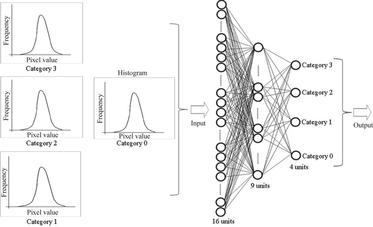
We used a feedforward ANN with a back propagation algorithm. On the first ANN for gray-level histograms, the ANN was composed of three layers consisting of input, hidden, and output layers. The ANN was composed of 16 input units, 9 hidden units, and 4 output units (Fig. 8). We used a total of 16 pieces (normalized frequency from 0 to 15 pixel values) on gray-level histograms as the input data (Fig. 2). The ANN was trained for the classification results (truth category = 0.9, other category = 0.1) [24]. In testing of ANN, when the output value was highest on the output unit of the truth category, the input data obtained from the ROI were considered as a truth category [24]. The first ANN for other texture features was composed of the same structure as the first ANN for gray-level histograms. As in the case of the first ANN for gray-level histograms, we used a total of 32 pieces (normalized frequency among ±16 pixel values), 32 pieces (16 normalized PS values for each of the principal and secondary axes), and 64 pieces (32 normalized PS values for each of the principal and secondary axes) as input data on the first ANN in the histogram of gray-level differences (Fig. 3), the GLRLM feature images (Fig. 5), and the GLCOM feature images (Fig. 7), respectively.
Fig. 8.
Architecture of training for the first ANN with gray-level histogram to classify the categories
Second ANN Combined with Four Texture Features
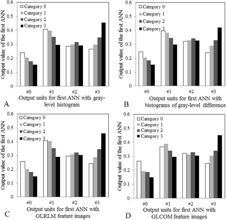
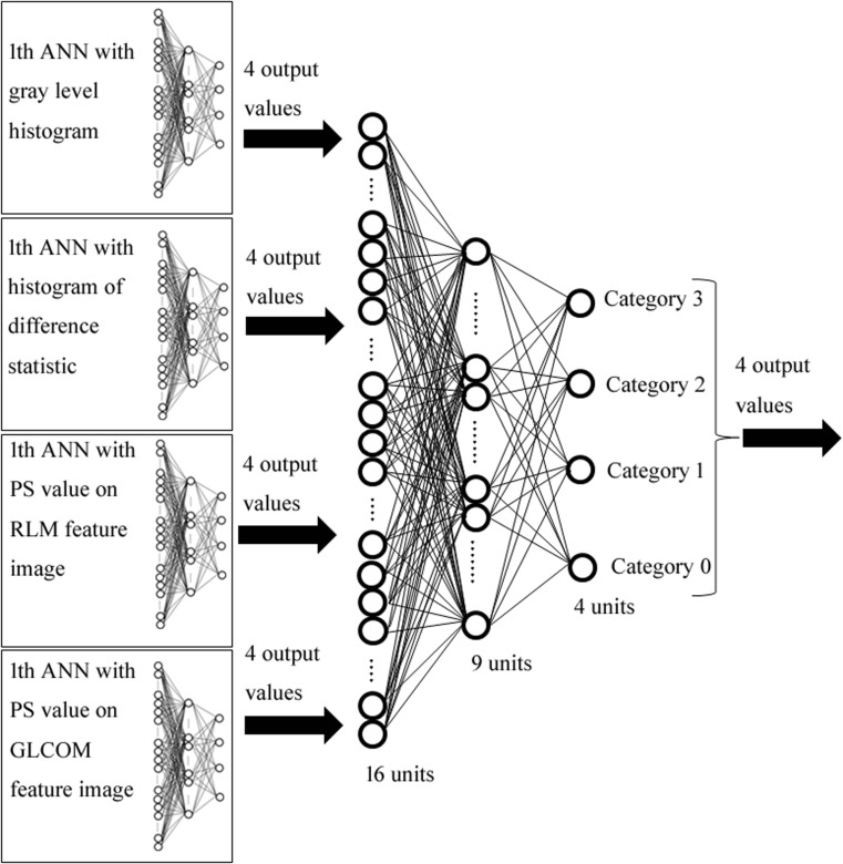
Figure 9 shows the output values obtained from the first ANN for each texture feature. On the output unit of category 0 (no. 0) on the gray-level histogram, the output value of category 0 was the highest of all categories (Fig. 9a). In addition, on the output unit of category 3 (no. 3) on the gray-level histogram, the output value of category 3 was the highest of all categories (Fig. 9a). Therefore, the second ANN was trained with output patterns obtained from the first ANN for each texture feature (Fig. 10). The second ANN was composed of 16 input units, 9 hidden units, and 4 output units. The input data consisted of a total of 16 pieces (four output values obtained from the first ANN with four texture features). In the same manner as the first ANN, the ANN was trained for the classification results (truth category = 0.9, other category = 0.1) [24].
Fig. 9.
Output values obtained from the first ANN for four texture features
Fig. 10.
Architecture of second ANN method for classification of pneumoconiosis category
Third ANN
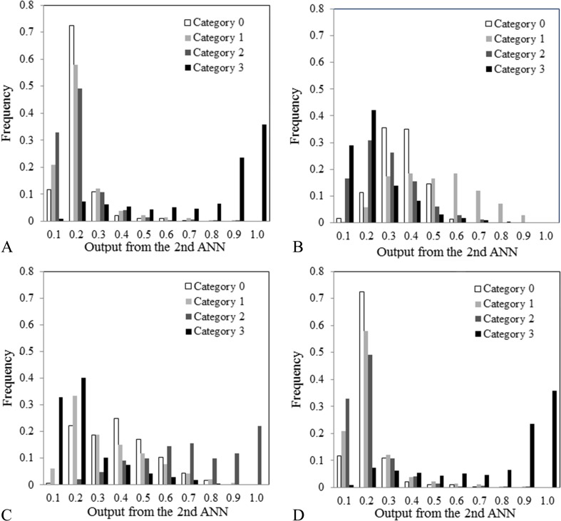
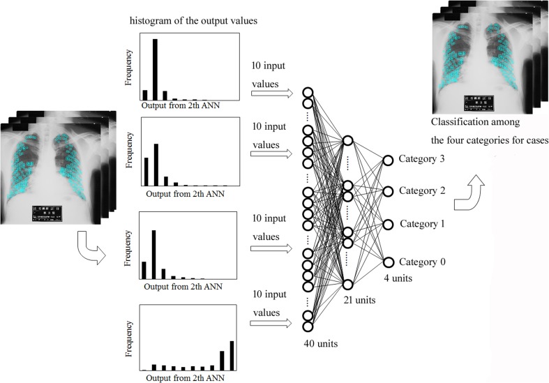
Figure 11 shows histograms of output values obtained from the second ANN for each case with four categories. Compared with the other categories, the histogram of category 1 was globally shifted to the right (Fig. 11b). In addition, the histogram of category 2 was globally shifted to the right (Fig. 11c). Therefore, for input data on the third ANN, we used a histogram of the output values obtained from the second ANN for each case (Fig. 12). The third ANN was composed of 40 input units, 21 hidden units, and 4 output units. Input data consisted of a total of 40 pieces (10 input values correspond to the 10 frequency values at 10 bins, from 0–0.1 to 0.9–1.0) [11]. In the same manner as the first and second ANN, the ANN was trained for the classification results (truth category = 0.9, other category = 0.1) [24].
Fig. 11.
Histograms of the output values obtained from the second ANN for each case with (a) category 0, (b) category 1, (c) category 2, and (d) category 3
Fig. 12.
Architecture of third ANN method for classification of pneumoconiosis category
Evaluation of Classification Performance
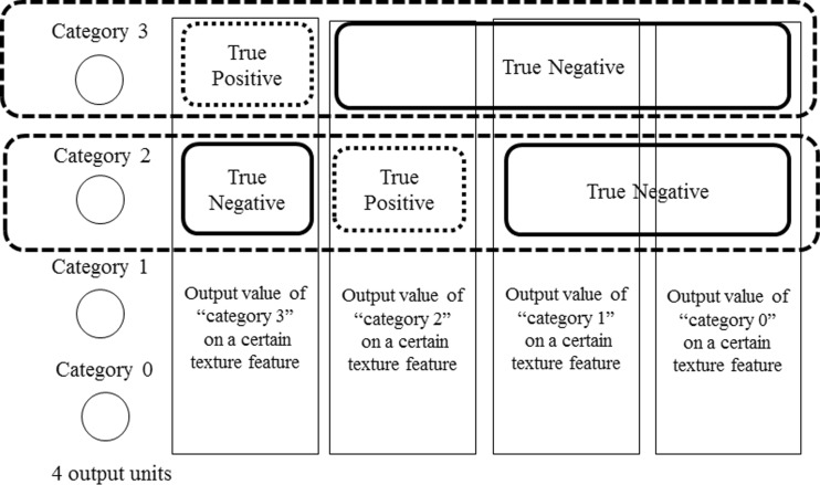
To investigate the effects of the number of gray levels and the distance level on each texture feature, we randomly divided the data into training data (category 0: 814 ROIs; category 1: 529 ROIs; category 2: 449 ROIs; and category 3: 544 ROIs) and non-training data (category 0: 813 ROIs; category 1: 528 ROIs; category 2: 449 ROIs; and category 3: 544 ROIs). We obtained averages of the ROC curves derived with the ten different pairs of non-training data sets. In addition, we calculated the statistical significance of differences between ROC curves using the two-tailed paired t test with each non-training data set. As shown in the Fig. 13, in the case of the ROC curve in category 3, the output values of “category 3” on a certain texture feature were regarded as “true positives,” the output values of the “other category” on a certain texture feature were regarded as “true negatives” [28]. We obtained the area under the ROC curve (AUC) on each category in this manner [28].
Fig. 13.
Classification method of four categories on ROC analysis
For evaluation of the classification performance with the third ANN method, the original database (category 0: 9 cases; category 1: 20 cases; category 2: 15 cases; and category 3: 11 cases) was divided randomly into training data and non-training data for each category. We obtained the case-based averages of the ROC curves derived with the ten different pairs of non-training data sets.
Results and Discussion
Effects of the Number of Gray Levels and the Distance Level of Texture Features
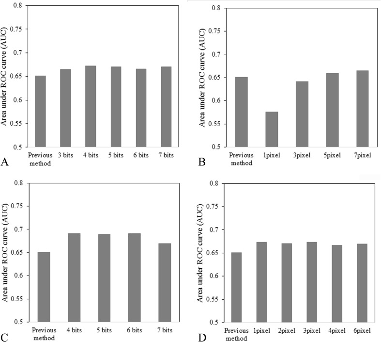
Figure 14 shows the effects of the number of gray levels and distance level on (a) the gray-level histogram, (b) the gray-level difference, (c) the GLRLM feature image, and (d) the GLCOM feature image in the first ANN. As shown in Fig. 14a, the classification performance with the gray-level histogram of the 4-bit gray level was greater than with the previous method (P < 0.05). As shown in Fig. 14b, the classification performance with the histogram of the gray-level difference (distance level: 7 pixels) was larger than with the previous method (P < 0.05). As shown in Fig. 14c, the classification performance with the GLRLM feature image on the 5-bit gray level was larger than with the previous method (P < 0.05). Finally, as shown in Fig. 14d, the classification performance with the GLCOM feature image (distance level: 3 pixels) was larger than with the previous method (P < 0.05).
Fig. 14.
Effects of the number of gray levels and distance level on (a) gray-level histogram, (b) gray-level difference, (c) GLRLM feature image, and (d) GLCOM feature image in the first ANN
With regard to the effect of the gray level, as the number of gray levels increased, the pixel values were spread and ungraded, and the texture features were decreased among the four categories [7]. On the other hand, as the gray level decreased, the pixel values were focused on some pixel value: these texture features were increased among the four categories [7]. With regard to the effect of the distance level, for segmentation of the lung in severe interstitial lung disease and for detection of diffuse lung disease on chest CT images, the distance level of GLCOM ranged from 0.50 to 0.89 mm [21, 31]. Therefore, we selected the gray-level histogram of the 4-bit gray level, the histogram of the gray-level difference on the 5-bit gray level and 7-pixel (1.23 mm) distance level, the GLRLM feature image on the 5-bit gray level, and the GLCOM feature image on the 6-bit gray level and 3-pixel (0.53 mm) distance level.
Classification Performance By Overall Scheme
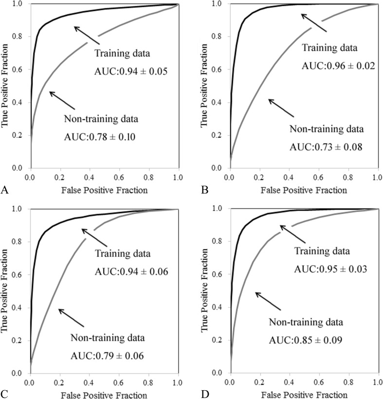
Figure 15 shows the ROC curves for (a) category 0, (b) category 1, (c) category 2, and (d) category 3 in the third ANN. Table 3 shows the AUC and specificity per case at 90% sensitivity obtained with the classification method using the third ANN for category 0, category 1, category 2, and category 3. On the non-training data, the AUC value and specificity for category 0 were 0.78 ± 0.10 and 34.2 ± 28.7%, respectively. The AUC value and specificity for category 1 were 0.73 ± 0.08 and 38.3 ± 11.7%, respectively. The AUC value and specificity for category 2 were 0.79 ± 0.06 and 52.5 ± 11.3%, respectively. The AUC value and specificity for category 3 were 0.85 ± 0.09 and 60.1 ± 24.9%, respectively. The AUC values for category 0, category 1, category 2, and category 3 were 0.72 ± 0.04, 0.59 ± 0.05, 0.51 ± 0.06, and 0.56 ± 0.05, respectively, on ROI-based performance with second ANN combined with the gray-level histograms, histograms of gray-level differences, GLRLM, and GLCOM feature images. However, use the histograms of output values obtained from the second ANN for each case suggested that the case performance with the third ANN was increased.
Fig. 15.
ROC curve on (a) category 0, (b) category 1, (c) category 2, and (d) category 3 in the third ANN
Table 3.
AUC and specificity per case at 90% sensitivity for third ANN in classifying among the four categories
| Training data | Non-training data | |||
|---|---|---|---|---|
| AUC | Specificity | AUC | Specificity | |
| Category 0 | 0.94 ± 0.05 | 80.7 ± 20.2% | 0.78 ± 0.10 | 34.2 ± 28.7% |
| Category 1 | 0.96 ± 0.02 | 89.5 ± 8.32% | 0.73 ± 0.08 | 38.2 ± 11.7% |
| Category 2 | 0.94 ± 0.06 | 88.4 ± 14.2% | 0.79 ± 0.06 | 52.5 ± 11.3% |
| Category 3 | 0.95 ± 0.03 | 90.3 ± 6.88% | 0.85 ± 0.09 | 60.1 ± 24.9% |
In a database including 300 normal and 125 pneumoconiosis cases (category 1, category 2, and category 3), Yu et al. reported that AUC value, sensitivity, and specificity were 0.978, 92.0, and 87.7%, respectively [15]. In addition, in a database including 85 normal and 40 pneumoconiosis cases (category 1 and category 2), Zhu et al. reported that AUC value, accuracy, sensitivity, and specificity were 0.974 ± 0.018 and 0.929 ± 0.018, 0.957 ± 0.021, and 0.873 ± 0.024, respectively [16]. However, the lower lung field of the right (AUC: 0.698) and left (AUC: 0.563) lungs that showed lower performance was not used [16]. Including our previous studies [31, 32], these CAD systems showed relatively high performance for detection of pneumoconiosis on chest radiographs. However, as our study involved classification among the four categories with four texture features and ANN simultaneously, it was difficult to compare the performance of classification of a number of cases, such as in our study, with previous studies that involved classification between two cases, such as normal vs. abnormal.
In the case of ANN for classification of a number of cases, the performance of ANN for differential diagnosis of interstitial lung disease on chest radiographs and diffuse lung disease on HRCT showed AUC for ANN performance of 0.911 and 0.956, respectively [27, 28]. As these previous studies used patient information (sex, age, etc.) and patient interview information (incubation period for symptoms, etc.) instead of radiological findings determined by radiologists, we suggest that the performance of the ANN for differential diagnosis was higher than in our study.
Without analyzing and extracting features of the images, it was useful for recognizing images with a convolutional neural network (CNN). The CNN was used for classification of interstitial lung disease and lung nodules on chest CT images [34, 35]. The CNN required many training times for detection of specific texture features. The input data for first ANN consisted of 16, 32, 32, and 64 pieces on gray-level histograms (as shown in Fig. 2), histograms of gray-level differences (as shown in Fig. 3), GLRLM (as shown in Fig. 5), and GLCOM feature images (as shown in Fig. 7), respectively. Our computerized method was classified among the four categories with less training time than the CNN.
Wang et al. created five GLRLM features for detection of diffuse lung disease patterns based on new GLRLMs: (1) the number of short runs with relatively high CT values, (2) the number of long runs with relatively high CT values, (3) the number of short runs with low CT values, (4) the number of long runs with low CT values, and (5) the total number of runs [21]. These CAD systems for detection of pneumoconiosis and diffuse lung disease used a combination of GLRLM and GLCOM features [15, 21]. By obtaining different texture features from the gray-level histogram, the histogram of the gray-level difference, the PS values on GLRLM, and GLCOM feature images, wherever the texture patterns were placed within the ROI, were thought to obtain adequate texture features.
In the future, as training of the ANN depends on the number of cases and texture types on pneumoconiosis, for evaluating the clinical efficacy of this CAD system, we will obtain a comprehensive database including a wide distribution of patterns for each category.
Conclusion
We have developed a three-stage ANN method combined with gray-level histograms, histograms of gray-level differences, GLRLM feature images, and GLCOM feature images for classification among the four categories with pneumoconiosis on chest radiography. Our computerized classification method will be useful in assisting radiologists in case-based classification of pneumoconiosis.
Compliance with Ethical Standards
Conflict of Interest
The authors declare that they have no conflict of interest.
Contributor Information
Eiichiro Okumura, Phone: +81-29-826-6000, Email: [email protected].
Ikuo Kawashita, Phone: +81-823-70-4566, Email: [email protected].
Takayuki Ishida, Phone: +81-6-6879-2573, Email: [email protected].
References
- 1.Fourth International Pneumoconiosis Conference: Report of the Working Party on the Definition of Pneumoconiosis. Geneva,1971
- 2.Guidelines for the use of ILO International Classification of Radiographs of Pneumoconiosis: Occupational Safety and Health Series, No.22 (Rev.), International Labor Office. Geneva,1980
- 3.Pneumoconiosis exploratory handbook: The Ministry of Labor Industrial Safety and Health Department industrial health division volume: Japan Industrial Safety and Health Association publication. Japan,1980
- 4.Chong S, Lee KS, Chung MJ, Han J, Kwon OJ, Kim TS. Pneumoconiosis: comparison of imaging and pathologic finding. Radiographics. 2006;26(1):59–77. doi: 10.1148/rg.261055070. [DOI] [PubMed] [Google Scholar]
- 5.Katsuragawa S, Doi K, MacMahon H. Image feature analysis and computer-aided diagnosis in digital radiography: detection and characterization of interstitial lung disease in digital chest radiographs. Med Phys. 1988;15:311–319. doi: 10.1118/1.596224. [DOI] [PubMed] [Google Scholar]
- 6.Katsuragawa S, Doi K, MacMahon H. Image feature analysis and computer-aided diagnosis in digital radiography: classification of normal and abnormal lungs with interstitial disease in chest images. Med Phys. 1989;16:38–44. doi: 10.1118/1.596412. [DOI] [PubMed] [Google Scholar]
- 7.Katsuragawa S, Doi K, Nakamori N, MacMahon H. Image feature analysis and computer-aided diagnosis in digital radiography: effect of digital parameters on the accuracy of computerized analysis of interstitial disease in digital chest radiographs. Med Phys. 1990;17:72–78. doi: 10.1118/1.596530. [DOI] [PubMed] [Google Scholar]
- 8.Katsuragawa S, Doi K, MacMahon H, Nakamori N, Sasaki Y, Fennessy JJ. Fennessy: quantitative computer-aided analysis of lung texture in chest radiographs. Radiographics. 1990;10:257–269. doi: 10.1148/radiographics.10.2.2326513. [DOI] [PubMed] [Google Scholar]
- 9.Katsuragawa S, Doi K, MacMahon H, Monnier-Cholley L, Ishida T, Kobayashi T. Classification of normal and abnormal lungs with interstitial diseases by rule-based method and artificial neural networks. J Digit Imaging. 1997;10:108–114. doi: 10.1007/BF03168597. [DOI] [PMC free article] [PubMed] [Google Scholar]
- 10.Ishida T, Katsuragawa S, Kobayashi T, MacMahon H, Doi K. Computerized analysis of interstitial disease in chest radiographs: improvement of geometric-pattern feature analysis. Med Phys. 1997;24:915–924. doi: 10.1118/1.598012. [DOI] [PubMed] [Google Scholar]
- 11.Ishida T, Katsuragawa S, Ashizawa K, MacMahon H, Doi K. Application of artificial neural networks for quantitative analysis of image data in chest radiographs for detection of interstitial lung disease. J Digit Imaging. 1998;11:182–192. doi: 10.1007/BF03178081. [DOI] [PMC free article] [PubMed] [Google Scholar]
- 12.Arzhaeva Y, Prokop M, Tax DM, De Jong PA, Schaefer-Prokop CM, van Ginneken B. Computer-aided detection of interstitial abnormalities in chest radiographs using a reference standard based on computed tomography. Med Phys. 2007;34:4798–4809. doi: 10.1118/1.2795672. [DOI] [PubMed] [Google Scholar]
- 13.Turner AF, Kruger RP, Thompson WB. Automated computer screening of chest radiographs for pneumoconiosis. Invest Radiol. 1976;11:258–266. doi: 10.1097/00004424-197607000-00002. [DOI] [PubMed] [Google Scholar]
- 14.Ledley RS, Huang HK, Rotolo LS. A texture analysis method in classification of coal workers’ pneumoconiosis. Comput Biol Med. 1975;5:53–67. doi: 10.1016/0010-4825(75)90018-9. [DOI] [PubMed] [Google Scholar]
- 15.Yu P, Xu H, Zhu Y, Yang C, Sun X, Zhao J. An automatic computer-aided detection scheme for pneumoconiosis on digital chest radiographs. J Digit Imaging. 2011;24:382–393. doi: 10.1007/s10278-010-9276-7. [DOI] [PMC free article] [PubMed] [Google Scholar]
- 16.Zhu B, Luo W, Li B, Chen B, Yang Q, Xu Y, Wu X, Chen H, Zhang K. The development and evaluation of a computerized diagnosis scheme for pneumoconiosis on digital chest radiographs. Biomed Eng Online. 2014;13:141. doi: 10.1186/1475-925X-13-141. [DOI] [PMC free article] [PubMed] [Google Scholar]
- 17.Zhu B, Chen H, Chen B, Xu Y, Zhang K. Support vector machine model for diagnosing pneumoconiosis based on wavelet texture features of digital chest radiographs. J Digit Imaging. 2014;27(1):90–97. doi: 10.1007/s10278-013-9620-9. [DOI] [PMC free article] [PubMed] [Google Scholar]
- 18.Delorme S, Keller-Reichenbecher MA, Zuna I, Schlegel W, Van Kaick G. Usual interstitial pneumonia. Quantitative assessment of high-resolution computed tomography findings by computer-assisted texture-based image analysis. Invest Radiol. 1997;32:566–574. doi: 10.1097/00004424-199709000-00009. [DOI] [PubMed] [Google Scholar]
- 19.Sluimer IC, van Waes PF, Viergever MA, van Ginneken B. Computer-aided diagnosis in high resolution CT of the lungs. Med Phys. 2003;30:3081–3090. doi: 10.1118/1.1624771. [DOI] [PubMed] [Google Scholar]
- 20.Uchiyama Y, Katsuragawa S, Abe H, Shiraishi J, Li F, Li Q, Zhang CT, Suzuki K, Doi K. Quantitative computerized analysis of diffuse lung disease in high-resolution computed tomography. Med Phys. 2003;30:2440–2454. doi: 10.1118/1.1597431. [DOI] [PubMed] [Google Scholar]
- 21.Wang J, Li F, Doi K, Li Q. Computerized detection of diffuse lung disease in MDCT: the usefulness of statistical texture features. Phys Med Biol. 2009;54:6881–6899. doi: 10.1088/0031-9155/54/22/009. [DOI] [PubMed] [Google Scholar]
- 22.Shiraishi J, Li Q, Suzuki K, Engelmann R, Doi K. Computer-aided diagnostic scheme for the detection of lung nodules on chest radiographs: localized search method based on anatomical classification. Med Phys. 2006;33:2642–2653. doi: 10.1118/1.2208739. [DOI] [PubMed] [Google Scholar]
- 23.Arimura H, Katsuragawa S, Suzuki K, Li F, Shiraishi J, Sone S, Doi K. Computerized scheme for automated detection of lung nodules in low-dose computed tomography images for lung cancer screening. Acad Radiol. 2004;11:617–629. doi: 10.1016/j.acra.2004.02.009. [DOI] [PubMed] [Google Scholar]
- 24.Suzuki K, Shiraishi J, Abe H, MacMahon H, Doi K. False-positive reduction in computer-aided diagnostic scheme for detecting nodules in chest radiographs by means of massive training artificial neural network. Acad Radiol. 2005;12:191–201. doi: 10.1016/j.acra.2004.11.017. [DOI] [PubMed] [Google Scholar]
- 25.Suzuki K, Armato SG, 3rd, Li F, Sone S, Doi K. Massive training artificial neural network (MTANN) for reduction of false positives in computerized detection of lung nodules in low-dose computed tomography. Med Phys. 2003;30:1602–1617. doi: 10.1118/1.1580485. [DOI] [PubMed] [Google Scholar]
- 26.Suzuki K, Li F, Sone S, Doi K. Computer-aided diagnostic scheme for distinction between benign and malignant nodules in thoracic low-dose CT by use of massive training artificial neural network. IEEE Trans Med Imaging. 2005;24:1138–1150. doi: 10.1109/TMI.2005.852048. [DOI] [PubMed] [Google Scholar]
- 27.Ashizawa K, MacMahon H, Ishida T, Nakamura K, Vyborny CJ, Katsuragawa S, Doi K. Effect of an artificial neural network on radiologists’ performance in the differential diagnosis of interstitial lung disease using chest radiographs. AJR Am J Roentgenol. 1999;172:1311–1315. doi: 10.2214/ajr.172.5.10227508. [DOI] [PubMed] [Google Scholar]
- 28.Fukushima A, Ashizawa K, Yamaguchi T, Matsuyama N, Hayashi H, Kida I, Imafuku Y, Egawa A, Kimura S, Nagaoki K, Honda S, Katsuragawa S, Doi K, Hayashi K. Application of an artificial neural network to high-resolution CT: usefulness in differential diagnosis of diffuse lung disease. AJR Am J Roentgenol. 2004;183:297–305. doi: 10.2214/ajr.183.2.1830297. [DOI] [PubMed] [Google Scholar]
- 29.Matake K, Yoshimitsu K, Kumazawa S, Higashida Y, Irie H, Asayama Y, Nakayama T, Kakihara D, Katsuragawa S, Doi K, Honda H. Usefulness of artificial neural network for differential diagnosis of hepatic masses on CT images. Acad Radiol. 2006;13:951–962. doi: 10.1016/j.acra.2006.04.009. [DOI] [PubMed] [Google Scholar]
- 30.Yamashita K, Yoshiura T, Arimura H, Mihara F, Noguchi T, Hiwatashi A, Togao O, Yamashita Y, Shono T, Kumazawa S, Higashida Y, Honda H. Performance evaluation of radiologists with artificial neural network for differential diagnosis of intra-axial cerebral tumors on MR images. AJNR Am J Neuroradiol. 2008;29:1153–1158. doi: 10.3174/ajnr.A1037. [DOI] [PMC free article] [PubMed] [Google Scholar]
- 31.Okumura E, Kawashita I, Ishida T. Computerized analysis of pneumoconiosis in digital chest radiography: effect of artificial neural network trained with power spectra. J Digit Imaging. 2011;24(6):1126–1132. doi: 10.1007/s10278-010-9357-7. [DOI] [PMC free article] [PubMed] [Google Scholar]
- 32.Okumura E, Kawashita I, Ishida T. Development of CAD based on ANN analysis of power spectra for pneumoconiosis in chest radiographs: effect of three new enhancement methods. Radiol Phys Technol. 2014;7(2):217–227. doi: 10.1007/s12194-013-0255-9. [DOI] [PMC free article] [PubMed] [Google Scholar]
- 33.Standard Radiographys of Pneumoconiosis . Electron Medium Edition. Japan: The Ministry of Labor; 2011. [Google Scholar]
- 34.Hua KL, Hsu CH, Hidayati SC, Cheng WH, Chen YJ. Computer-aided classification of lung nodules on computed tomography images via deep learning technique. Onco Targets Ther. 2015;8:2015–2022. doi: 10.2147/OTT.S80733. [DOI] [PMC free article] [PubMed] [Google Scholar]
- 35.Anthimopoulos M, Christodoulidis S, Ebner L, Christe A, Mougiakakou S. Lung pattern classification for interstitial lung diseases using a deep convolutional neural network. IEEE Trans Med Imaging. 2016;35(5):1207–1216. doi: 10.1109/TMI.2016.2535865. [DOI] [PubMed] [Google Scholar]


