Exact sampling of the unobserved covariates in Bayesian spline models for measurement error problems

Anindya Bhadra; Raymond J Carroll

doi:10.1007/s11222-015-9572-7

. Author manuscript; available in PMC: 2016 Jul 12.

Published in final edited form as: Stat Comput. 2015 Jun 14;26(4):827–840. doi: 10.1007/s11222-015-9572-7

Exact sampling of the unobserved covariates in Bayesian spline models for measurement error problems

Anindya Bhadra ^1,^✉, Raymond J Carroll ²

PMCID: PMC4941830 NIHMSID: NIHMS701628 PMID: 27418743

Abstract

In truncated polynomial spline or B-spline models where the covariates are measured with error, a fully Bayesian approach to model fitting requires the covariates and model parameters to be sampled at every Markov chain Monte Carlo iteration. Sampling the unobserved covariates poses a major computational problem and usually Gibbs sampling is not possible. This forces the practitioner to use a Metropolis–Hastings step which might suffer from unacceptable performance due to poor mixing and might require careful tuning. In this article we show for the cases of truncated polynomial spline or B-spline models of degree equal to one, the complete conditional distribution of the covariates measured with error is available explicitly as a mixture of double-truncated normals, thereby enabling a Gibbs sampling scheme. We demonstrate via a simulation study that our technique performs favorably in terms of computational efficiency and statistical performance. Our results indicate up to 62 and 54 % increase in mean integrated squared error efficiency when compared to existing alternatives while using truncated polynomial splines and B-splines respectively. Furthermore, there is evidence that the gain in efficiency increases with the measurement error variance, indicating the proposed method is a particularly valuable tool for challenging applications that present high measurement error. We conclude with a demonstration on a nutritional epidemiology data set from the NIH-AARP study and by pointing out some possible extensions of the current work.

Keywords: Bayesian methods, Gibbs sampling, Measurement error models, Nonparametric regression, Truncated normals

1 Introduction

Nonparametric regression problems where the covariates are measured with error have received considerable attention in the statistics literature. Carroll et al. (1999) proposed a semi-parametric estimator based on the SIMEX method of Cook and Stefanski (1994) and a parametric estimator assuming that the unobserved covariates can be represented via a mixture of normals. Carroll et al. (2004) established important identifiability results for estimating the model parameters under mild conditions. In related developments in a Bayesian framework, Berry et al. (2002) established a fully Bayesian approach to fit spline models to measurement error problems as an attractive computational alternative to the SIMEX-based approach of Carroll et al. (1999) and the iterative conditional modes (ICM) approach of Besag (1986). In simulations, the Bayesian approach of Berry et al. (2002) demonstrated marked performance improvement over competing methods. Carroll et al. (2004) and Ganguli et al. (2005) extended the Bayesian approach presented by Berry et al. (2002). Detailed discussion on software implementation for fitting Bayesian penalized spline models can be found in Crainiceanu et al. (2005).

However, in fully Bayesian approaches, sampling the unobserved covariates measured with error requires a Metropolis–Hastings step. Designing a Metropolis–Hastings sampler requires careful tuning and is known to be difficult in high dimensions, often resulting in slow convergence of the sampler (Roberts and Rosenthal 2001). This has been recognized as a major computational hindrance to practical Bayesian approaches to fitting nonparametric regression models in measurement error problems (Berry et al. 2002; Carroll et al. 2004), and the complete conditional distribution of the unobserved covariates measured with error has been intractable so far. In some of the more recent works, Marley and Wand (2010) demonstrated the computational aspects and implementation of a Bayesian semi-parametric regression in presence of missing data and measurement error using the BRugs software package that uses an underlying Metropolis–Hastings step for the unobserved covariates. Alternatively, Pham et al. (2013) considered an approximate sampling technique via a grid-based mean field variational Bayes approach to sample from a tractable approximation of the posterior of the unobserved covariates in a measurement error problem. This can be useful in a number of situations and might provide a reasonable approximation of the posterior. However, unlike Markov chain Monte Carlo (MCMC) approaches, such mean field approximations do not sample from the exact posterior distribution as the target distribution of a Markov chain and can lead to inconsistent parameter estimates under certain situations, for example, in state-speace models (Wang and Titterington 2004).

It is generally recognized that when available, the Gibbs sampler enjoys a number of advantages over alternative MCMC techniques (Gelfand and Smith 1990). It requires no tuning and samples are not rejected since they come from the complete conditional distributions. To the practitioner, the benefits enjoyed by the Gibbs sampler often make it the default choice among the full repertoire of MCMC techniques. However, establishing a Gibbs sampler has so far not been possible for the unobserved covariates in a Bayesian setting using splines. In this article, we offer an exact sampling procedure for the covariates measured with error for truncated polynomial and B-splines of degree equal to one, resulting in a Gibbs sampler. In both cases, we establish the required conditional posterior as a mixture of double-truncated normal distributions. Efficient sampling from a truncated normal distribution has itself been a source of investigation by multiple researchers in the statistics literature, with a naive rejection sampling method replaced by an efficient implementation by Robert (1995) and improved upon further by Chopin (2011). We use Chopin’s implementation of the truncated normal sampler and apply it to draw our required conditional posterior samples. We conduct a simulation study where we compare performances of the SIMEX-based technique of Carroll et al. (1999) and the Metropolis–Hastings approach of Berry et al. (2002) versus Gibbs sampling using the complete conditional posterior, and establish the superior statistical and computational properties of our method. Specifically, we demonstrate that the proposed method results in up to 62 and 54 % increase in mean integrated squared error efficiency over the method of Berry et al. (2002) while using truncated polynomial splines and B-splines respectively. We also obtain far greater efficiency compared to non-Bayesian approaches. We find evidence that the gain in efficiency increases with the measurement error variance and thus the proposed method is particularly suited for difficult problems with high measurement error.

We apply the proposed technique to a nutritional epidemiology data set arising from the NIH-AARP Diet and Health Study (http://dietandhealth.cancer.gov). Such data are usually collected via food frequency questionnaires (FFQ) and are well-known to be prone to high measurement error. We again find evidence of superior performance of the proposed techniques over the technique of Berry et al. (2002).

The rest of the article is organized as follows: in Sect. 2, we start out by providing the necessary background on Bayesian approaches to measurement error models. We then establish the Gibbs samplers for the cases where a degree-one truncated polynomial spline and a degree-one B-spline are used. Implementational issues of number and placement of knots for spline models are described in Sect. 2.3. We provide an outline of the SIMEX-based approach in Sect. 2.4 which serves as the basis of comparison of the proposed Bayesian technique with non-Bayesian alternatives. In Sect. 2.5 we provide the necessary background for efficiently sampling from a truncated normal distribution that appears in our Gibbs sampler. We conduct a simulation study detailing the performances of the competing methods in Sect. 3 and discuss the application on the NIH-AARP data in Sect. 4. We conclude by pointing out several possible extensions in Sect. 5.

2 Bayesian approaches to spline models for measurement error problems

Consider the measurement error model

Y_{i} = g (X_{i}) + ε_{i},

(1)

W_{i j} = X_{i} + U_{i j}, j = 1, \dots, m_{i}, i = 1, \dots, n,

(2)

where n is the sample size and m_i is the number of replicates for individual i for i = 1, …, n. We assume ε_i are independent and identically distributed normal random variables with mean 0 and variance $σ_{ε}^{2}$ ; U_{i j} are independent and identically distributed normal random variables with mean 0 and variance $σ_{u}^{2}$ ; U_ij and ε_i are uncorrelated; and g(·) is the true, unknown, smooth, mean function. The observed data are the pairs (Y_i, W_i₁, …, W_{im_i}) while X_i are unobserved and hence latent. An efficient approach for modeling g(·) to approximate it to a desired degree of smoothness is via penalized truncated polynomial splines (P-splines) or B-splines bases (Eilers and Marx 1996). The chief advantage of using penalized P-splines or B-splines over smoothing splines is that one needs the number of basis functions to be equal to the number of knot points for penalized P-splines; and equal to the number of internal knots + degree + 1 for penalized B-splines. Whereas, the number of basis functions is equal to the number of data points for smoothing splines, which can be large. Ruppert and Carroll (2000) and Berry et al. (2002) showed that via an appropriate choice of normally distributed priors over the spline coefficients, one can penalize the sum of squared jumps at the knots to control the degree of smoothness in a Bayesian implementation of P-splines. If a degree one truncated polynomial spline is used to model g(·), the set of basis functions is given by B(x) = {1, x, B₁(x), …, B_K (x)} where

B_{k} (x) = {(x - ω_{k})}_{+},

(3)

for k = 1, …, K, where ω₁, …, ω_K are the known knot points. The complete Bayesian hierarchical model can then be described as

Y_{i} = β_{0} + β_{1} X_{i} + \sum_{k = 1}^{K} B_{k} (X_{i}) θ_{k} + ε_{i},

(4)

W_{i j} = X_{i} + U_{i j},

(5)

\begin{array}{l} ε_{i} ~ Normal (0, σ_{ε}^{2}), U_{i j} ~ Normal (0, σ_{u}^{2}), \\ X_{i} ~ Normal (μ_{x}, σ_{x}^{2}), \end{array}

(6)

where we assume the following conjugate prior distribution on the parameters:

\begin{array}{l} μ_{x} ~ Normal (0, σ_{μ_{x}}^{2}); σ_{x}^{2} ~ IG (a_{x}, b_{x}); \\ σ_{u}^{2} ~ IG (a_{u}, b_{u}); σ_{ε}^{2} ~ IG (a_{ε}, b_{ε}); \end{array}

and the priors on the spline coefficients are given by

\begin{array}{l} β_{0}, β_{1} ~ Normal (0, σ_{β}^{2} I_{2}); \\ θ_{1}, \dots, θ_{K} ~ Normal (0, σ_{θ}^{2} I_{K}) . \end{array}

(7)

Define $M = \sum_{i = 1}^{n} m_{i}, W_{i •} = \sum_{j = 1}^{m_{i}} W_{i j}$ , W̄_i_• = W_i_•/m_i, Θ = (β₀, β₁, θ₁, …, θ_K)^T and let IG(a, b) denote an inverse gamma distribution with shape parameter a and scale parameter b. For this model, Berry et al. (2002) showed that the posterior mean for the fit has the same expression as the penalized P-spline fit of Eilers and Marx (1996) for $σ_{β}^{2} \to \infty$ and in practice one can use a large value for that parameter. They also derived the posteriors of all the model parameters in closed form and specified the complete conditionals required for Gibbs sampling. These are available through standard algebraic manipulations and we report them here for the sake of completeness. In particular, they derived that

μ_{x} ∣ rest ~ Normal {{(n σ_{x}^{- 2} + σ_{μ_{x}}^{- 2})}^{- 1} n \bar{X} σ_{x}^{- 2}, {(n σ_{x}^{- 2} + σ_{μ_{x}}^{- 2})}^{- 1}},

(8)

σ_{x}^{2} ∣ rest ~ IG (a_{x} + n / 2, b_{x} + \frac{1}{2} \sum_{i = 1}^{n} {(X_{i} - μ_{x})}^{2}),

(9)

σ_{u}^{2} ∣ rest ~ IG (a_{u} + M / 2, b_{u} + \frac{1}{2} \sum_{i = 1}^{n} {(W_{i •} - m_{i} X_{i})}^{2}),

(10)

σ_{ε}^{2} ∣ rest ~ IG (a_{ε} + n / 2, b_{ε} + \frac{1}{2} \sum_{i = 1}^{n} {(Y_{i} - β_{0} - β_{1} X_{i} - \sum_{k = 1}^{K} B_{k} (X_{i}))}^{2}),

(11)

Θ ∣ rest ~ Normal {{(σ_{ε}^{- 2} Z^{T} Z + diag (σ_{β}^{- 2} I_{2}, σ_{θ}^{- 2} I_{K}))}^{- 1} Z^{T} Y σ_{ε}^{- 2}, {(σ_{ε}^{- 2} Z^{T} Z + diag (σ_{β}^{- 2} I_{2}, σ_{θ}^{- 2} I_{K}))}^{- 1}},

(12)

where the n × (K + 2) matrix Z is given by

Z = [\begin{matrix} 1 & X_{1} & B_{1} (X_{1}) & \dots & B_{K} (X_{1}) \\ ⋮ & ⋮ & ⋮ & ⋱ & ⋮ \\ 1 & X_{n} & B_{1} (X_{n}) & \dots & B_{K} (X_{n}) \end{matrix}] .

However, they resorted to a Metropolis–Hastings step for the unobserved X_i and commented on the associated computational difficulties due to convergence problems of the sampler and careful tuning necessary to design a good candidate density. Therefore, it is worth investigating whether it is possible to design a Gibbs sampler for X_i. We show this is indeed the case for truncated polynomial splines or B-splines of degree equal to one in the hierarchical setting specified above.

The model using B-spline bases is similar, even though this was not treated in the works of Berry et al. (2002) or Carroll et al. (2004). In this case, the basis does not include an intercept and X_i and therefore we do not need the terms β₀ and β₁ in Eq. (4) and they can be set to 0. Also, unlike truncated polynomial splines, B-splines are defined on a compact support. For measurement error problems, one needs to choose this support judiciously so that the unobserved covariate X_i has negligible probability of lying outside this interval. A reasonable choice is [min_i (W̄_i_•), max_i (W̄_i_•)]. Set ω₀ to be the minimum of this support and ω_K to be the maximum of the support. Let (ω₁, …, ω_K₋₁) be K − 1 internal knots. The set of K + 1 degree one B-spline basis functions is now B̃(x) = {B̃₁(x), …, B̃_K₊₁(x)} where

{\tilde{B}}_{1} (x) = \frac{ω_{1} - x}{ω_{1} - ω_{0}} 1 (ω_{0} \leq x < ω_{1}),

(13)

{\tilde{B}}_{K + 1} (x) = \frac{x - ω_{K - 1}}{ω_{K} - ω_{K - 1}} 1 (ω_{K - 1} \leq x < ω_{K}),

(14)

and

{\tilde{B}}_{k} (x) = \frac{x - ω_{k - 2}}{ω_{k - 1} - ω_{k - 2}} 1 (ω_{k - 2} \leq x < ω_{k - 1}) + \frac{ω_{k} - x}{ω_{k} - ω_{k - 1}} 1 (ω_{k - 1} \leq x < ω_{k}),

(15)

for k = 2, …, K. The other difference is that, according to Eilers and Marx (1996), the prior on the corresponding (K + 1) parameter vector Θ is now

θ_{1}, \dots, θ_{K + 1} ~ Normal (0, σ_{θ}^{2} P^{-}),

(16)

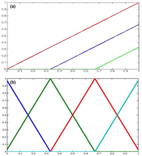
where for a first order difference penalty $P = D_{1}^{T} D_{1}$ , where D₁ is the matrix representation of the first difference operator. Computational details for this operator are described in the appendix of Eilers and Marx (1996). Here P⁻ is the generalized inverse of P. With these changes, the calculations of the posteriors of the parameters have forms very similar to the case of truncated polynomial splines. Figure 1 plots the basis functions for degree 1 truncated polynomial splines and B-splines in the interval [0, 1]. The choice of basis functions has received a lot of attention in nonparametric literature and detailed discussion can be found, for example, in Hastie and Tibshirani (1990). We do not treat these issues further in this article. Instead, we focus on our main finding: that any measurement error model with additive Gaussian error terms where the basis functions contain terms that are only linear in the unobserved covariate X_i, the complete conditional distribution of X_i follows a mixture of truncated normal random variables. Below, we formalize our results in the form of two propositions that give the parameters and the mixture proportions associated with the truncated normals for truncated polynomial splines and B-splines respectively. The proofs of the propositions are given in Appendix A. Numerical results are discussed in Sect. 3.

Fig. 1 — a Degree 1 P-spline basis functions on [0, 1] with knots at 0, 0.33 and 0.67 and b degree 1 B-spline basis functions on [0, 1] with two interior knots at 0.33 and 0.67. For both a and b, each *distinct color* indicates one basis function. (Color figure online)

2.1 Complete conditional distribution for X_i for degree one truncated polynomial splines

We now consider the case where degree one truncated polynomial splines of Eq. (3) are used as basis functions. Define the sequence of knots (ω₁, …, ω_K) along with the convention that ω₀ = −∞ and ω_K ₊₁ = ∞. In this case, the following proposition establishes the required conditional as a mixture of double-truncated normal distributions:

Proposition 1 (Truncated polynomial splines of degree 1)

Define

\begin{array}{l} ζ_{1 i L} = {{(σ_{ε}^{2})}^{- 1} {(β_{1} + \sum_{ℓ = 1}^{L} θ_{ℓ})}^{2} + m_{i} / (σ_{u}^{2}) + 1 / (σ_{x}^{2})}^{- 1}; \\ ζ_{2 i L} = - {(2 σ_{ε}^{2})}^{- 1} {- 2 β_{1} Y_{i} - 2 Y_{i} \sum_{ℓ = 1}^{L} θ_{ℓ} + 2 (β_{0} - \sum_{ℓ = 1}^{L} θ_{ℓ} ω_{ℓ}) (β_{1} + \sum_{ℓ = 1}^{L} θ_{ℓ})} + (W_{i •} / σ_{u}^{2} + μ_{x} / σ_{x}^{2}); \\ ζ_{3 i L} = - {(2 σ_{ε}^{2})}^{- 1} {2 Y_{i} \sum_{ℓ = 1}^{L} θ_{i} ω_{ℓ} + {(β_{0} - \sum_{ℓ = 1}^{L} θ_{ℓ} ω_{ℓ})}^{2}} . \end{array}

Further define

\begin{array}{l} b_{i L} = (ω_{L + 1} - ζ_{1 i L} ζ_{2 i L}) / \sqrt{ζ_{1 i L}}; \\ a_{i L} = (ω_{L} - ζ_{1 i L} ζ_{2 i L}) / \sqrt{ζ_{1 i L}}; \\ D_{i} = {[\sum_{L = 0}^{K} {Φ (b_{i L}) - Φ (a_{i L})} exp {(1 / 2) \log (ζ_{1 i L}) + ζ_{3 i L} + ζ_{1 i L} {(ζ_{2 i L})}^{2} / 2}]}^{- 1}; \\ p_{i L} = D_{i} {Φ (b_{i L}) - Φ (a_{i L})} exp {(1 / 2) \log (ζ_{1 i L}) + ζ_{3 i L} + ζ_{1 i L} {(ζ_{2 i L})}^{2} / 2} \\ = D_{i} \sqrt{ζ_{1 i L}} {Φ (b_{i L}) - Φ (a_{i L})} \times exp {ζ_{3 i L} + ζ_{1 i L} {(ζ_{2 i L})}^{2} / 2} . \end{array}

Then, the complete conditional distribution of X_i is a mixture of truncated normal random variables on the intervals [ω_L, ω_L₊₁] for L = 0, …, K, with means ζ_i₁_L ζ_i₂_L, variances ζ_i₁_L and with mixing probabilities p_iL.

Proof

See Appendix A.1.

2.2 Complete conditional distribution for X_i for degree one B-splines

Define the compact interval [ω₀, ω_K] with K − 1 internal knots (ω₁, …, ω_K ₋₁). Let the K + 1 degree ones B-splines basis functions B̃_k (X_i), used to model g(·), be defined by Eqs. (13–15). Use the convention ω₋₁ = −∞, ω_K₊₁ = ∞ and θ₀ = θ_K ₊₂ = 0. Then our results are similar to Proposition 1 and the required conditional is again a mixture of double-truncated normal distributions.

Proposition 2 (B-splines of degree 1)

Define

\begin{array}{l} {\tilde{ζ}}_{1 i L} = {[{(σ_{ε}^{2})}^{- 1} {\frac{θ_{L + 2} - θ_{L + 1}}{ω_{L + 1} - ω_{L}}}^{2} + m_{i} / (σ_{u}^{2}) + 1 / (σ_{x}^{2})]}^{- 1}; \\ {\tilde{ζ}}_{2 i L} = - {(2 σ_{ε}^{2})}^{- 1} {- 2 (\frac{θ_{L + 2} - θ_{L + 1}}{ω_{L + 1} - ω_{L}}) Y_{i} + 2 (\frac{ω_{L + 1} θ_{L + 1} - ω_{L} θ_{L + 2}}{ω_{L + 1} - ω_{L}}) (\frac{θ_{L + 2} - θ_{L + 1}}{ω_{L + 1} - ω_{L}})} + (W_{i •} / σ_{u}^{2} + μ_{x} / σ_{x}^{2}); \\ {\tilde{ζ}}_{3 i L} = - {(2 σ_{ε}^{2})}^{- 1} {- 2 Y_{i} \frac{ω_{L + 1} θ_{L + 1} - ω_{L} θ_{L + 2}}{ω_{L + 1} - ω_{L}} + {(\frac{ω_{L + 1} θ_{L + 1} - ω_{L} θ_{L + 2}}{ω_{L + 1} - ω_{L}})}^{2}} . \end{array}

Further define

\begin{array}{l} {\tilde{b}}_{i L} = (ω_{L + 1} - {\tilde{ζ}}_{1 i L} {\tilde{ζ}}_{2 i L}) / \sqrt{{\tilde{ζ}}_{1 i L}}; \\ {\tilde{a}}_{i L} = (ω_{L} - {\tilde{ζ}}_{1 i L} {\tilde{ζ}}_{2 i L}) / \sqrt{{\tilde{ζ}}_{1 i L}}; \\ {\tilde{D}}_{i} = {[\sum_{L = 0}^{K} {Φ ({\tilde{b}}_{i L}) - Φ ({\tilde{a}}_{i L})} exp {(1 / 2) \log ({\tilde{ζ}}_{1 i L}) + {\tilde{ζ}}_{3 i L} + {\tilde{ζ}}_{1 i L} {({\tilde{ζ}}_{2 i L})}^{2} / 2}]}^{- 1}; \\ {\tilde{p}}_{i L} = {\tilde{D}}_{i} {Φ ({\tilde{b}}_{i L}) - Φ ({\tilde{a}}_{i L})} exp {(1 / 2) \log ({\tilde{ζ}}_{1 i L}) + {\tilde{ζ}}_{3 i L} + {\tilde{ζ}}_{1 i L} {({\tilde{ζ}}_{2 i L})}^{2} / 2} \\ = D_{i} \sqrt{{\tilde{ζ}}_{1 i L}} {Φ ({\tilde{b}}_{i L}) - Φ ({\tilde{a}}_{i L})} \times exp {{\tilde{ζ}}_{3 i L} + {\tilde{ζ}}_{1 i L} {({\tilde{ζ}}_{2 i L})}^{2} / 2} . \end{array}

Then, the complete conditional distribution of X_i is a mixture of truncated normal random variables on the intervals [ω_L, ω_L₊₁] for L = −1, …, K, with means ζ̃_i₁_L ζ̃_i₂_L, variances ζ̃_i₁_L and with mixing probabilities p̃_iL.

Proof

See Appendix A.2.

Remark 1

Whereas both propositions result in similar distributions for the unobserved covariates, there are also important differences. In particular, while for B-splines the mean and the standard deviation of the unobserved covariates in a given interval depend only on the spline coefficients at the two neighboring knots, for truncated polynomial splines they depend on all the previous knots as well. The mixing probabilities follow the same pattern.

Remark 2

The major difference in the implementation of truncated polynomial splines and B-splines is the prior on the spline coefficients from Eqs. (7) and (16). Whereas for truncated polynomial splines, we follow the choice of prior according to Sect. 2.1 of Berry et al. (2002), for B-splines we follow the specification given in Eilers and Marx (1996). While Eilers and Marx (1996) did not consider a Bayesian approach, our choice of prior results in a posterior mean for the spline coefficients that coincides with the penalized B-splines estimates in Eq. (13) of Eilers and Marx (1996). For all the other parameters, our choice of priors coincides with Berry et al. (2002).

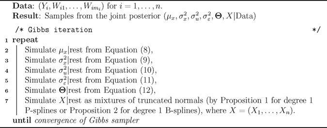
The explicit conditionals for the unobserved covariates X now enables a full Gibbs sampler for Bayesian spline models in measurement error problems (as opposed to Metropolis–Hastings within Gibbs). Algorithm 1 summarizes all the required steps in the proposed sampler.

Algorithm 1.

Gibbs sampler for Bayesian spline models for measurement error problems

graphic file with name nihms701628f7.jpg

Open in a new tab

2.3 Selection of number and placement of knots

The problem of selection and placement of knots have received a lot of attention in nonparametrics literature. However, as noted in Ruppert (2002) and Carroll et al. (2004), provided that the number of knots is more than a certain minimum, the exact number of knots has relatively little effect on the fit compared to that of the smoothing parameter in the case of P-splines. We find similar numerical behavior and our proposed estimator is quite robust to the number of knots, once about 20 knots have been used. We experimented with equally placed knots and knots placed on the sample quantiles of the observed noisy covariate and again find that this has relatively little effect on the fit. We also note that the results presented in Propositions 1 and 2 do not make any assumptions about the placement of knots.

2.4 Alternatives to Bayesian techniques: the simulation-extrapolation (SIMEX) approach

We compare the proposed Bayesian technique to the SIMEX technique of Cook and Stefanski (1994) and in this section we give a description of the SIMEX algorithm. As noted in Carroll et al. (2004), the SIMEX method needs a base model that results from considering the case where there is no measurement error and the resultant estimators in this case form the base estimates. Similar to Carroll et al. (2004), one can then apply the iterations of the SIMEX method with the estimated ${\hat{σ}}_{u}^{2}$ for the measurement error variance and simulated Normal(0, $ξ {\hat{σ}}_{u}^{2}$ ) terms added to W in in each iteration of the method for ξ > 0. Of course ξ needs to be bigger than 0 for the variance term to be defined. The idea of the SIMEX method is to plot the resultant estimates against ξ and extrapolate to ξ = −1. The asymptotic justifications for the SIMEX method are described in Stefanski and Cook (1995) and Carroll et al. (1996) and we refer the interested readers to the references therein. In addition to comparing performance of our proposed technique to the Bayesian technique utilizing MCMC as in Carroll et al. (2004), we also provide numerical performance comparisons with the SIMEX method in Sect. 3.

2.5 Simulating from a double-truncated normal distribution

While the closed-form expression for the complete conditional for X_i as a mixture of double-truncated normals in Propositions 1 and 2 is an interesting analytic result, its practical usefulness depends of course on how efficiently such random variables can be simulated. A simple rejection sampling scheme to simulate a normal random variable truncated from the left at a is as follows: generate a sample X_i from a standard Gaussian, accept the sample if X_i > a. While this approach has at least 50 % acceptance rate if a < 0, it obviously performs poorly for large positive values of a. A more efficient algorithm was proposed by Robert (1995) who used a rejection sampling scheme with an exponential proposal density and outlined the steps to choose the parameter of the proposal density in order to achieve the optimal acceptance rate. Chopin (2011) proposed another approach where one essentially samples a random digit and then performs a table look-up to simulate the required truncated normal random variable where the entries of the table have been pre-computed. This approach achieves up to two-fold speedup over Robert (1995). There are other possible approaches for simulating from a truncated normal and while Chopin (2011) is our method of choice for the purpose of this article, we refer the interested reader to the references therein for a performance comparison of various truncated normal samplers.

3 Simulation study

Our simulation example is similar to one of the examples of Carroll et al. (2004). Specifically, we consider the true mean function to be

g (x) = \frac{3 sin (π x / 2)}{1 + 2 x^{2} {sign (x) + 1}},

where sign(x) = 1 if x > 0 and 0 otherwise. We sample X_i from Normal(0, $σ_{x}^{2}$ ). To generate the simulated data according to Eqs. (1–2), we use n = 500, m_i = 2, $σ_{x}^{2} = 1.0$ and $σ_{ε}^{2} = 0.09$ . We consider four values of $σ_{u}^{2}$ , equal to 0.33, 0.5, 0.75 and 1.0 respectively, progressively increasing the measurement error.

We compare the performances of four approaches: a “naive” smoothing spline fit ignoring the measurement error, the SIMEX approach of Cook and Stefanski (1994), a Bayesian approach with random walk Metropolis–Hastings algorithm for X_i due to Berry et al. (2002) and our Bayesian approach with truncated normal sampling from the complete conditional of X_i. To do this, we generate 100 simulated data sets with the parameter values specified above and compute the sum of squared deviations between the true mean curve and the fitted means for each method, computed on the interval [−2, 2] on an equally-spaced 101 grid points. In each case, the Bayesian approaches far outperform the naive fit and SIMEX. In order to compare performance of the two Bayesian approaches, we let the sampler run for approximately 10 seconds. We verify that this results in good mixing in both the cases. With the same computing time, it is possible to perform about 3000 Metropolis–Hastings iterations and about 300 iterations of the truncated normal sampler, i.e., Metropolis–Hastings is about 10 times faster. However, the truncated normal sampling generates samples from the full conditional posterior as part of a Gibbs step, so there is no chance of a sample getting rejected and unlike Metropolis–Hastings, no tuning is necessary. Therefore, it seems interesting to compare performances of the two Bayesian approaches.

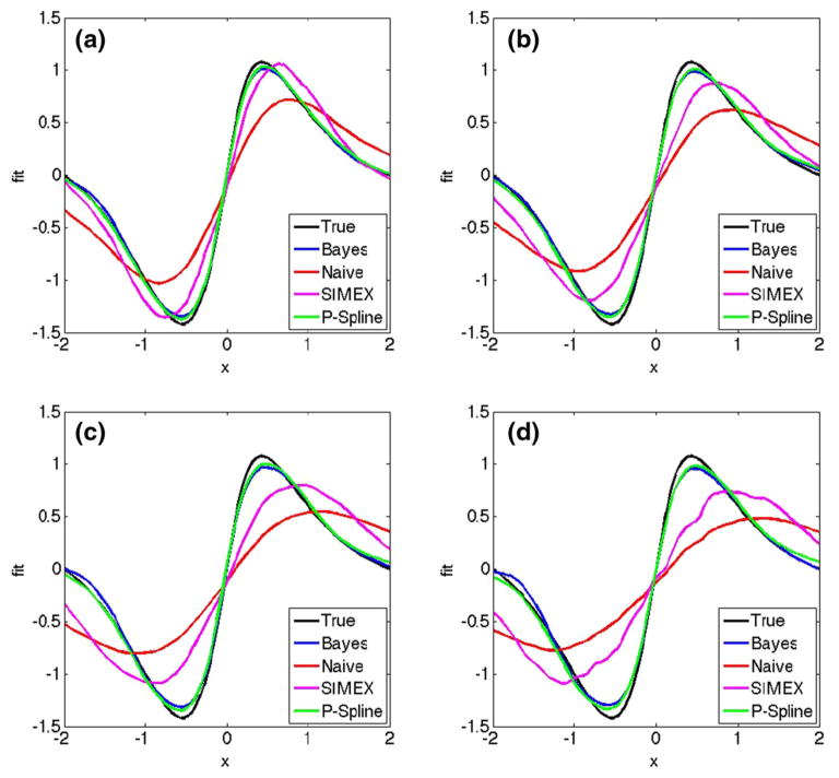
The results using truncated polynomial splines are summarized in Table 1, where we compute the mean integrated squared error efficiency of the Bayesian fit with truncated normal sampling compared to the other methods, defined as the ratio of average integrated squared error for the competing methods divided by the average integrated squared error for Bayesian fit with truncated normal sampling, where the average is computed over the 100 simulated data sets. For the splines, we use 25 knots and place them evenly on the sample quantiles of W̄_i_•. We see that for Metropolis–Hastings, the acceptance rate of the sampler is around 69–74 % for the different scenarios, which is much higher than the theoretically optimal 23.4 % acceptance rate suggested by Roberts et al. (1997) for random walk Metropolis algorithms, leading us to believe the sampler of Berry et al. (2002) is slow to converge. One must also note that the figure of 23.4 % given by Roberts et al. (1997) is an asymptotic result and in a given problem, while it is well-known that both very high and very low acceptance rates indicate poor performance of Metropolis–Hastings, it remains a major challenge to design good proposals. Figure 2 shows the average fitted mean curves for the different approaches. We observe from Table 1 that for the same computing time, the truncated normal sampler provides improved performance as the measurement error variance increases, with between 18–62 % increase in mean integrated squared error efficiency over the Bayesian method using Metropolis–Hastings, and of course has much greater efficiency than the naive fit or SIMEX.

Table 1.

Mean integrated squared error efficiency of the Bayesian fit with truncated normal sampling (“Bayes-TN-Psplines”) compared to the naive fit ignoring measurement error, SIMEX, and the Bayesian fit with Metropolis–Hastings (“Bayes (M–H)”). In each case $σ_{x}^{2} = 1.0$

σ_{u}^{2} / σ_{x}^{2}

0.33

0.50

0.75

1.00

Time (s)

Naive

14.23

16.43

19.55

15.91

0.004

SIMEX

9.34

10.35

14.33

14.43

0.027

Bayes (M–H)

1.33 (74.0)

1.18 (72.8)

1.56 (70.2)

1.62 (69.0)

9.904

Open in a new tab

The numbers in parentheses for “Bayes M–H” is the percentage of proposals accepted by the sampler. Computing times are based on MATLAB programs running on a Macintosh with a 3.1 GHz Intel processor and 16 GB of RAM

Fig. 2 — Plot of the true mean function and the fitted mean curves averaged over 100 simulated data sets for $σ_{x}^{2} = 1.0$ and $σ_{u}^{2} / σ_{x}^{2}$ values (a) 0.33, (b) 0.50, (c) 0.75 and (d) 1.00. Each panel shows the true curve (*black*), the mean for naive fit (*red*), the mean for SIMEX fit (*purple*), the mean for Bayesian fit with Metropolis–Hastings (*blue*) and the mean for Bayesian fit with truncated normal sampling using P-splines (*green*). (Color figure online)

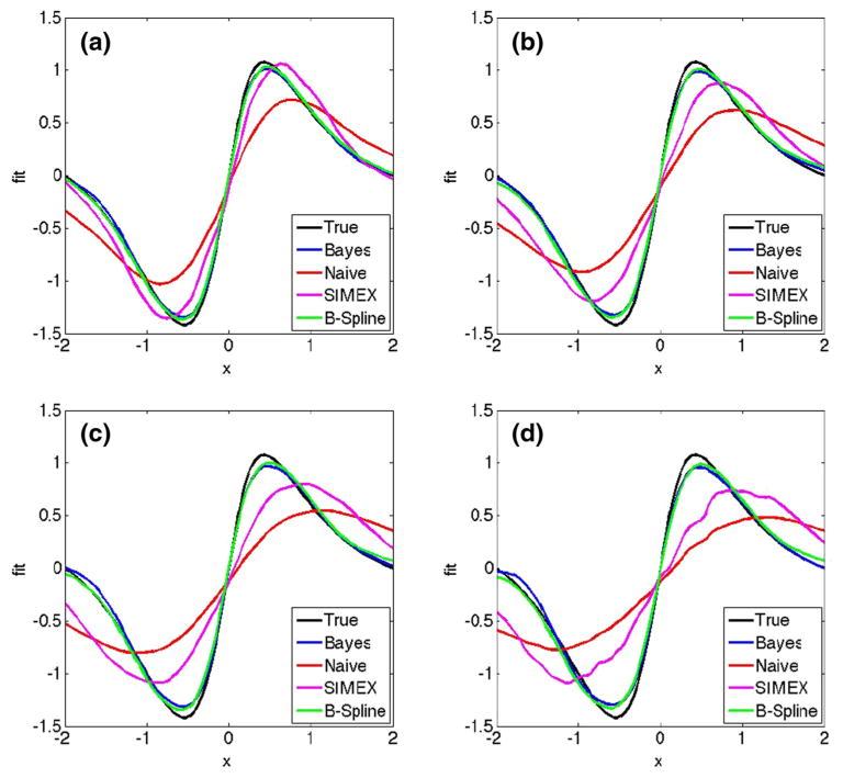
We provide performance comparisons when B-spline basis functions are used in Table 2. We have used the same number of knots as before, but the knots are now equally placed between the minimum and maximum of W̄_i_• due to the ease of computing the B-spline basis functions on equally spaced knots. We see that the truncated normal sampler again outperforms SIMEX and the naive method quite easily. Furthermore, we see an improvement between 13 and 54 % over Bayesian approach with Metropolis–Hastings. Figure 3 shows the average fitted mean curve for the competing methods in this case. We verified that the placement of the knots, whether evenly placed or placed on sample quantiles of W̄_i_•, has relatively little effect on the fit.

Table 2.

Mean integrated squared error efficiency of the Bayesian fit with truncated normal sampling (“Bayes-TN-Bsplines”) compared to the naive fit ignoring measurement error, SIMEX, and the Bayesian fit with Metropolis–Hastings (“Bayes (M–H)”). In each case $σ_{x}^{2} = 1.0$

σ_{u}^{2} / σ_{x}^{2}

0.33

0.50

0.75

1.00

Time (seconds)

Naive

12.81

15.61

19.40

14.59

0.005

SIMEX

8.41

9.83

14.22

13.23

0.035

Bayes (M-H)

1.20 (74.0)

1.13 (70.9)

1.54 (70.5)

1.49 (69.0)

10.214

Open in a new tab

Fig. 3 — Plot of the true mean function and the fitted mean curves averaged over 100 simulated data sets for $σ_{x}^{2} = 1.0$ and $σ_{u}^{2} / σ_{x}^{2}$ values (a) 0.33, (b) 0.50, (c) 0.75 and (d) 1.00. Each panel shows the true curve (*black*), the mean for naive fit (*red*), the mean for SIMEX fit (*purple*), the mean for Bayesian fit with Metropolis–Hastings (*blue*) and the mean for Bayesian fit with truncated normal sampling using B-splines (*green*). (Color figure online)

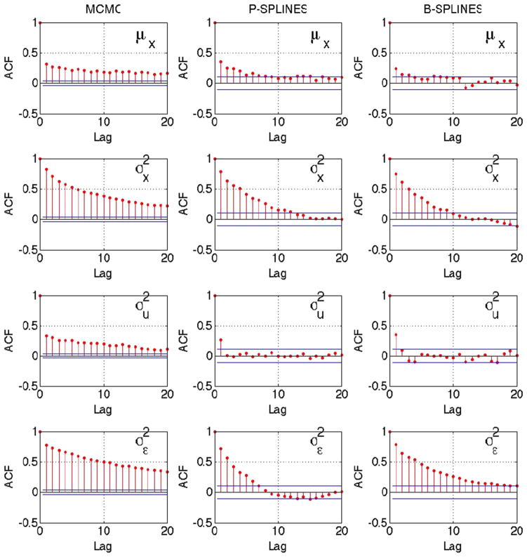
In Figure 4 we plot the sample autocorrelation function (ACF) of the parameters μ_x, $σ_{x}^{2}, σ_{u}^{2}$ and $σ_{ε}^{2}$ for the Bayesian approaches with Metropolis–Hastings and the Gibbs sampling based approaches. For each of the parameters, the ACF shows faster decay while using the proposed approach compared to Metropolis–Hastings. This indication of better mixing with the proposed approach, especially when the measurement error variance is high, provides a justification for the improved performance seen in terms of the mean integrated squared error efficiency in Tables 1 and 2.

Fig. 4 — Sample autocorrelation plot of selected parameters for Bayesian method with Metropolis–Hastings MCMC (*left*), truncated normal sampler with P-splines (*center*) and truncated normal sampler with B-splines (*right*) for simulated data. Truncated normal sampler improves mixing for both P-splines and B-splines. True $σ_{u}^{2} = 1.0$

Therefore, our main finding from the simulation study is that sampling the unobserved covariates from the complete conditionals can result in major computational advantages over Metropolis–Hastings for Bayesian treatment to spline models in measurement error problems. This resultant technique offers significant improvement in mean integrated squared error efficiency. There is evidence that this increase in efficiency is more pronounced as the measurement noise variance $σ_{u}^{2}$ increases, i.e., the proposed method performs better for more difficult problems. In contrast, the choice of basis functions (truncated polynomial splines versus B-splines) or the placement and number of knots do not appear to have a substantial effect on the fit.

Remark 3

MATLAB code for the simulation example is freely available on the website of the first author at http://www.stat.purdue.edu/~bhadra/software.html as a .zip archive. A README file documents the use of the software.

4 Application on the NIH-AARP diet and health study data

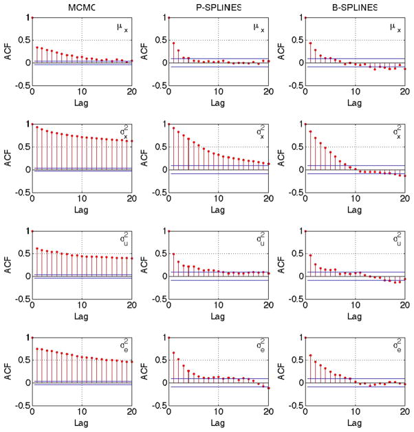
To demonstrate the performance of the proposed methodology, we consider the nutritional epidemiology data analyzed previously by Sinha et al. (2010). The motivating data arises from the NIH-AARP Diet and Health Study (http://dietandhealth.cancer.gov) and the details can be found in Schatzkin et al. (2001). In large scale nutritional epidemiology studies such as this, it is customary to measure the dietary intake of the individuals via a food frequency questionnaire (FFQ). However, the FFQ, which may span over several months, is well-known to be subject to substantial measurement error (Thompson and Subar 2001; Thomson et al. 2003). In order to adjust for the measurement error in the FFQ, the NIH-AARP study includes a calibration study of approximately 2000 men and women who are administered two consecutive 24-h recalls, when they are interviewed on their dietary intakes over the past 24 h. Among the subjects of the calibration study, we specifically focus on the women who completed both the 24-h recall interviews, leaving us with n = 934 subjects. We define Y_i = log(% of non alcohol energy from total fat in the FFQ) and W_ij = log(% of non alcohol energy from total fat in the 24-h recall) for individual i in recall j. The reason to focus on the fat energy intake is that this has been suspected to play a role in several types of cancer. Figure 5 plots the calibrated fit θ_cal(x) against x obtained using the three Bayesian methods (Metropolis–Hastings, truncated polynomial splines and B-splines). The three Bayesian methods result in almost identical fits, which are quite similar to Fig. 2 of Sinha et al. (2010). The departure from the dashed y = x straight line in the figure provides evidence of a nonlinear effect in the fit, justifying the need for using a flexible non-parametric model. Figure 6 plots the sample ACF for the parameters μ_x, $σ_{x}^{2}, σ_{u}^{2}$ and $σ_{ε}^{2}$ and once again, the Gibbs samplers show evidence of better mixing over Metropolis–Hastings for all the parameters.

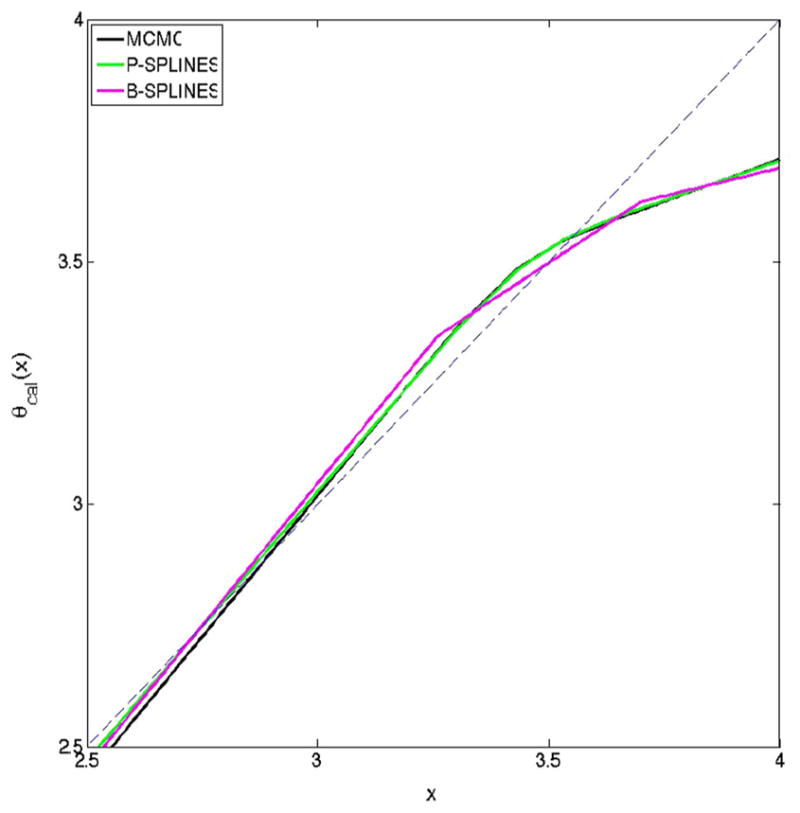
Fig. 5 — Fit for the NIH-AARP calibration study data for women using the Bayesian methods with Metropolis–Hastings MCMC, Gibbs sampler with P-splines and Gibbs sampler with B-splines. The broken straight line has intercept zero and slope one

Fig. 6 — Sample autocorrelation plot of selected parameters for Bayesian method with Metropolis–Hastings MCMC (*left*), truncated normal sampler with P-splines (*center*) and truncated normal sampler with B-splines (*right*) for the NIH-AARP calibration study data. Truncated normal sampler improves mixing for both P-splines and B-splines

5 Conclusions

We propose a computationally attractive method for fitting spline models of degree one in measurement error problems. In a conjugate prior setting, we establish the required complete conditional distribution of the unobserved covariates as a mixture of double-truncated normals, thus enabling Gibbs sampling for the unobserved covariates using efficient simulation techniques for truncated normals. The gain in mean integrated squared error efficiency over competing approaches is substantial and there is evidence that the gain increases with the measurement error variance, i.e., as the problem becomes more challenging. This is perhaps not surprising since designing an efficient Metropolis–Hastings sampler in such settings is difficult. Though we have not investigated it in this article, another case where one might expect to see the benefit of the proposed approach over Metropolis–Hastings is with high-dimensional unobserved covariates. Though our technique does not generalize to splines of degree more than one, we note that in many cases splines of lower degree provide adequate performance in terms of smoothing and interpolation of highly nonlinear functions, such as the true mean function considered in our simulation example. In fact, they may actually be preferred over splines of higher degree, since fewer coefficients need to be estimated. We demonstrate that the proposed technique is applicable to degree one truncated polynomial splines and B-splines and it is in fact true to that similar results can be found whenever the basis functions consist of degree one terms in the unobserved covariate X_i, regardless of the exact form of the basis function. Thus, it is not hard to see that the technique presented in this article could be easily extended to additive models of multiple covariates and to nonparametric regression models involving tensor products of truncated power basis functions, as examples of two immediate possible extensions of the current work. Furthermore, the technique could also be extended to mixture models, specifically where the covariates can be represented as a mixture of normals or the responses can be represented as a normal location scale-mixture. It is therefore quite reasonable to expect our technique to be an important addition to the toolbox of the practitioners working with measurement error problems and to stimulate future research in the directions identified above.

Acknowledgments

Carroll’s research was supported by Grant U01-CA057030 from the National Cancer Institute.

Appendix A: Proofs of Proposition 1 and 2

Recall that Θ denotes the (K + 2) parameter vector (β₀, β₁, θ₁, …, θ_K)^T. The log likelihood of the complete data is given by

\begin{array}{l} ℒ = - {(2 σ_{ε}^{2})}^{- 1} {(Y - Z Θ)}^{T} (Y - Z Θ) - (n / 2) log (σ_{ε}^{2}) \\ - (K / 2) log (σ_{θ}^{2}) - {(2 σ_{θ}^{2})}^{- 1} \sum_{k = 1}^{K} θ_{k}^{2} - (a_{ε} + 1) log (σ_{ε}^{2}) \\ - (a_{θ} + 1) log (σ_{θ}^{2}) - (b_{ε} / σ_{ε}^{2}) - (b_{θ} / σ_{θ}^{2}) \\ - {(2 σ_{u}^{2})}^{- 1} \sum_{i = 1}^{n} \sum_{j = 1}^{m_{i}} {(W_{i j} - X_{i})}^{2} - (N / 2) log (σ_{u}^{2}) \\ - {(2 σ_{x}^{2})}^{- 1} \sum_{i = 1}^{n} {(X_{i} - μ_{x})}^{2} - (n / 2) log (σ_{x}^{2}) \\ - (a_{x} + 1) log (σ_{x}^{2}) - (a_{u} + 1) log (σ_{u}^{2}) - b_{x} / σ_{x}^{2} \\ - b_{u} / σ_{u}^{2} - μ_{x}^{2} / (2 σ_{μ}^{2}) - {(2 σ_{β}^{2})}^{- 1} (β_{0}^{2} + β_{1}^{2}) + constant, \end{array}

where “constant” is a collection of all terms that are independent of data as well as model parameters. Collecting the terms containing X in Inline graphic , except for an irrelevant constant,

ℒ_{x} = - {(2 σ_{ε}^{2})}^{- 1} (- Θ^{T} Z^{T} Y - Y^{T} Z Θ + Θ^{T} Z^{T} Z Θ) - {(2 σ_{u}^{2})}^{- 1} \sum_{i = 1}^{n} \sum_{j = 1}^{m_{i}} {(W_{i j} - X_{i})}^{2} - {(2 σ_{x}^{2})}^{- 1} \sum_{i = 1}^{n} {(X_{i} - μ_{x})}^{2} .

We also have

Θ^{T} Z^{T} Y = Y^{T} Z Θ = β_{0} \sum_{i = 1}^{n} Y_{i} + β_{1} \sum_{i = 1}^{n} X_{i} Y_{i} + \sum_{i = 1}^{n} \sum_{k = 1}^{K} θ_{k} B_{k} (X_{i}) Y_{i}

and

Θ^{T} Z^{T} Z Θ = \sum_{i = 1}^{n} {β_{0} + β_{1} X_{1} + \sum_{k = 1}^{K} θ_{k} B_{k} (X_{i})}^{2} .

Thus in Inline graphic the terms corresponding to X_i are

ℒ_{x_{i}} = - {(2 σ_{ε}^{2})}^{- 1} [- 2 X_{i} β_{1} Y_{i} - 2 Y_{i} \sum_{k = 1}^{K} θ_{k} B_{k} (X_{i}) + {β_{0} + β_{1} X_{i} + \sum_{k = 1}^{K} θ_{k} B_{k} (X_{i})}^{2}] - {(2 σ_{u}^{2})}^{- 1} \sum_{j = 1}^{m_{i}} {(W_{i j} - X_{i})}^{2} - {(2 σ_{x}^{2})}^{- 1} {(X_{i} - μ_{x})}^{2} .

(17)

Recall that $W_{i •} = \sum_{j = 1}^{m_{i}} W_{i j}$ . In the next two subsections, we treat the special cases of polynomial splines of degree 1 and B-splines of degree 1 respectively.

A.1 Proof of Proposition 1

In this case, the basis functions are given by Eq. (3). We now establish the distribution of each X_i given all the other quantities as a mixture of truncated normals. To see this, suppose ω_L ≤ X_i < ω_L₊₁ where 0 ≤ L ≤ K with the convention that ω₀ = −∞, ω_K₊₁ = ∞ and (X_i − ω₀)₊ = X_i. From Equation (17), when ω_L ≤ X_i < ω_L₊₁, we have

\sum_{k = 1}^{K} θ_{k} B_{k} (X_{i}) = \sum_{ℓ = 1}^{L} θ_{ℓ} (X_{i} - ω_{ℓ}),

and the relevant terms in the log likelihood for X_i are

\begin{array}{l} ℒ_{x_{i}}^{L} = - {(2 σ_{ε}^{2})}^{- 1} [- 2 X_{i} β_{1} Y_{i} - 2 Y_{i} \sum_{ℓ = 1}^{L} θ_{ℓ} (X_{i} - ω_{ℓ}) \\ + {β_{0} + β_{1} X_{i} + \sum_{ℓ = 1}^{L} θ_{ℓ} (X_{i} - ω_{ℓ})}^{2}] \\ - X_{i}^{2} {m_{i} / (2 σ_{u}^{2}) + 1 / (2 σ_{x}^{2})} + X_{i} (W_{i •} / σ_{u}^{2} + μ_{x} / σ_{x}^{2}) \\ = - {(2 σ_{ε}^{2})}^{- 1} [- 2 X_{i} β_{1} Y_{i} - 2 Y_{i} \sum_{ℓ = 1}^{L} θ_{ℓ} (X_{i} - ω_{ℓ}) \\ + {(β_{0} - \sum_{ℓ = 1}^{L} θ_{ℓ} ω_{ℓ}) + X_{i} (β_{1} + \sum_{ℓ = 1}^{L} θ_{ℓ})}^{2}] \\ - X_{i}^{2} {m_{i} / (2 σ_{u}^{2}) + 1 / (2 σ_{x}^{2})} + X_{i} (W_{i •} / σ_{u}^{2} + μ_{x} / σ_{x}^{2}) \\ = X_{i}^{2} {- {(2 σ_{ε}^{2})}^{- 1} {(β_{1} + \sum_{ℓ = 1}^{L} θ_{ℓ})}^{2} - m_{i} / (2 σ_{u}^{2}) - 1 / (2 σ_{x}^{2})} \\ + X_{i} [- {(2 σ_{ε}^{2})}^{- 1} {- 2 β_{1} Y_{i} \\ - 2 Y_{i} \sum_{ℓ = 1}^{L} θ_{ℓ} + 2 (β_{0} - \sum_{ℓ = 1}^{L} θ_{ℓ} ω_{ℓ}) (β_{1} + \sum_{ℓ = 1}^{L} θ_{ℓ})} \\ + (W_{i •} / σ_{u}^{2} + μ_{x} / σ_{x}^{2})] \\ - {(2 σ_{ε}^{2})}^{- 1} {2 Y_{i} \sum_{ℓ = 1}^{L} θ_{ℓ} ω_{ℓ} + {(β_{0} - \sum_{ℓ = 1}^{L} θ_{ℓ} ω_{ℓ})}^{2}} \\ = - {(2 ζ_{1 i L})}^{- 1} X_{i}^{2} + ζ_{2 i L} X_{i} + ζ_{3 i L} . \end{array}

Thus, the density function of X_i is

\begin{array}{l} f_{X_{i}} (x) \propto \sum_{L = 0}^{K} I (ω_{L} \leq x \leq ω_{L + 1}) \times exp {- x^{2} / (2 ζ_{1 i L}) + ζ_{2 i L} x + ζ_{3 i L}} \\ = \sum_{L = 0}^{K} I (ω_{L} \leq x \leq ω_{L + 1}) \times exp {- \frac{{(x - ζ_{1 i L} ζ_{2 i L})}^{2}}{2 ζ_{1 i l}} + ζ_{3 i L} + ζ_{1 i L} {(ζ_{2 i L})}^{2} / 2} \\ \propto \sum_{L = 0}^{K} I (ω_{L} \leq x \leq ω_{L + 1}) \frac{1}{\sqrt{2 π ζ_{1 i L}}} \times exp {- \frac{{(x - ζ_{1 i L} ζ_{2 i L})}^{2}}{2 ζ_{1 i L}}} \times exp {(1 / 2) log (ζ_{1 i L}) + ζ_{3 i L} + ζ_{1 i L} {(ζ_{2 i L})}^{2} / 2} . \end{array}

(18)

This shows the density of X_i on the interval [ω_L, ω_L₊₁] is proportional to a double-truncated normal with mean ζ₁_iLζ₂_iL and variance ζ₁_iL, truncated at the boundaries and the overall density for X_i is a mixture of (K + 1) of these truncated normals, since 0 ≤ L ≤ K, giving (K + 1) mixture components. From Eq. (18), we see that the mixing probabilities p_iL ∝ {Φ(b_iL) − Φ(a_iL)} exp {(1/2)log(ζ₁_iL) + ζ₃_iL + ζ₁_iL (ζ₂_iL)² /2}. Further note that it must hold that $\sum_{L = 0}^{K} p_{i L} = 1$ , so all that remains is to find the appropriate normalizations for the p_iL. By algebra, we see that

f_{X i} (x) = D_{i} \sum_{L = 0}^{K} I (ω_{L} \leq x \leq ω_{L + 1}) \times \frac{1}{\sqrt{2 π ζ_{1 i L}}} exp {- \frac{{(x - ζ_{1 i L} ζ_{2 i L})}^{2}}{2 ζ_{1 i L}}} \times exp {(1 / 2) log (ζ_{1 i L}) + ζ_{3 i L} + ζ_{1 i L} {(ζ_{2 i L})}^{2} / 2} .

Again by algebra, we see that the mixing probabilities then become p_iL, as claimed.

A.2 Proof of Proposition 2

In this case, the (K + 1) basis functions are given by Eqs. (13–15) and β₀ = β₁ = 0. We again establish the distribution of each X_i given all the other quantities as a mixture of truncated normals. The fitted function is

\sum_{k = 1}^{K + 1} θ_{k} {\tilde{B}}_{k} (X_{i}) = \sum_{k = 1}^{K + 1} 1 (ω_{k - 1} \leq X_{i} < ω_{k}) \times {\frac{X_{i} - ω_{k - 1}}{ω_{k} - ω_{k - 1}} θ_{k + 1} + \frac{ω_{k} - X_{i}}{ω_{k} - ω_{k - 1}} θ_{k}} .

Clearly, if X_i < ω₀ or X_i ≥ ω_K then $\sum_{k = 1}^{K + 1} θ_{k} {\tilde{B}}_{k} (X_{i}) = 0$ . For L = 0, …, K − 1, suppose ω_L ≤ X_i < ω_L₊₁. Then the relevant terms in the log likelihood for X_i are

\begin{array}{l} ℒ_{x_{i}}^{L} = - {(2 σ_{ε}^{2})}^{- 1} [- 2 Y_{i} X_{i} \frac{θ_{L + 2} - θ_{L + 1}}{ω_{L + 1} - ω_{L}} \\ - 2 Y_{i} \frac{ω_{L + 1} θ_{L + 1} - ω_{L} θ_{L + 2}}{ω_{L + 1} - ω_{L}} \\ + {\frac{ω_{L + 1} θ_{L + 1} - ω_{L} θ_{L + 2}}{ω_{L + 1} - ω_{L}} + X_{i} \frac{θ_{L + 2} - θ_{L + 1}}{ω_{L + 1} - ω_{L}}}^{2}] \\ - X_{i}^{2} {m_{i} / (2 σ_{u}^{2}) + 1 / (2 σ_{x}^{2})} + X_{i} (W_{i •} / σ_{u}^{2} + μ_{x} / σ_{x}^{2}) \\ = X_{i}^{2} [- {(2 σ_{ε}^{2})}^{- 1} {\frac{θ_{L + 2} - θ_{L + 1}}{ω_{L + 1} - ω_{L}}}^{2} - m_{i} / (2 σ_{u}^{2}) - 1 / (2 σ_{x}^{2})] \\ + X_{i} [- {(2 σ_{ε}^{2})}^{- 1} {- 2 (\frac{θ_{L + 2} - θ_{L + 1}}{ω_{L + 1} - ω_{L}}) Y_{i} \\ + 2 (\frac{ω_{L + 1} θ_{L + 1} - ω_{L} θ_{L + 2}}{ω_{L + 1} - ω_{L}}) (\frac{θ_{L + 2} - θ_{L + 1}}{ω_{L + 1} - ω_{L}})} \\ + (W_{i •} / σ_{u}^{2} + μ_{x} / σ_{x}^{2})] \\ - {(2 σ_{ε}^{2})}^{- 1} {- 2 Y_{i} \frac{ω_{L + 1} θ_{L + 1} - ω_{L} θ_{L + 2}}{ω_{L + 1} - ω_{L}} \\ + {(\frac{ω_{L + 1} θ_{L + 1} - ω_{L} θ_{L + 2}}{ω_{L + 1} - ω_{L}})}^{2}} \\ = - {(2 {\tilde{ζ}}_{1 i L})}^{- 1} X_{i}^{2} + {\tilde{ζ}}_{2 i L} X_{i} + {\tilde{ζ}}_{3 i L} . \end{array}

If X_i < ω₀ or X_i ≥ ω_K the the relevant terms in the log likelihood are

- X_{i}^{2} {m_{i} / (2 σ_{u}^{2}) + 1 / (2 σ_{x}^{2})} + X_{i} (W_{i •} / σ_{u}^{2} + μ_{x} / σ_{x}^{2}) .

Then, by calculations similar to Appendix A.1, the proof of Proposition 2 is completed.

Contributor Information

Anindya Bhadra, Email: [email protected].

Raymond J. Carroll, Email: [email protected].

References

Berry SM, Carroll RJ, Ruppert D. Bayesian smoothing and regression splines for measurement error problems. J Am Stat Assoc. 2002;97:160–169. [Google Scholar]
Besag J. On the statistical analysis of dirty pictures. J R Stat Soc Ser B. 1986;48:259–302. [Google Scholar]
Carroll RJ, Kchenhoff H, Lombard F, Stefanski LA. Asymptotics for the simex estimator in nonlinear measurement error models. J Am Stat Assoc. 1996;91:242–250. [Google Scholar]
Carroll RJ, Maca JD, Ruppert D. Nonparametric regression in the presence of measurement error. Biometrika. 1999;86:541–554. [Google Scholar]
Carroll RJ, Ruppert D, Crainiceanu CM, Tosteson TD, Karagas MR. Nonlinear and nonparametric regression and instrumental variables. J Am Stat Assoc. 2004;99:736–750. [Google Scholar]
Chopin N. Fast simulation of truncated Gaussian distributions. Stat Comput. 2011;21:275–288. [Google Scholar]
Cook JR, Stefanski LA. Simulation-extrapolation estimation in parametric measurement error models. J Am Stat Assoc. 1994;89:1314–1328. [Google Scholar]
Crainiceanu CM, Ruppert D, Wand MP. Bayesian analysis for penalized spline regression using WinBUGS. J Stat Softw. 2005;14:1–24. [Google Scholar]
Eilers PHC, Marx BD. Flexible smoothing with B-splines and penalties. Stat Sci. 1996;11:89–121. [Google Scholar]
Ganguli B, Staudenmayer J, Wand M. Additive models with predictors subject to measurement error. Aust N Z J Stat. 2005;47:193–202. [Google Scholar]
Gelfand AE, Smith AFM. Sampling-based approaches to calculating marginal densities. J Am Stat Assoc. 1990;85:398–409. [Google Scholar]
Hastie TJ, Tibshirani RJ. Generalized Additive Models. CRC Press; Boca Raton: 1990. [Google Scholar]
Marley JK, Wand MP. Non-standard semiparametric regression via BRugs. J Stat Softw. 2010;37:1–30. [Google Scholar]
Pham TH, Ormerod JT, Wand MP. Mean field variational Bayesian inference for nonparametric regression with measurement error. Comput Stat Data Anal. 2013;68:375–387. [Google Scholar]
Robert C. Simulation of truncated normal variables. Stat Comput. 1995;5:121–125. [Google Scholar]
Roberts GO, Gelman A, Gilks WR. Weak convergence and optimal scaling of random walk Metropolis algorithms. Annals Appl Probab. 1997;7:110–120. [Google Scholar]
Roberts GO, Rosenthal JS. Optimal scaling for various Metropolis–Hastings algorithms. Stat Sci. 2001;16:351–367. [Google Scholar]
Ruppert D. Selecting the number of knots for penalized splines. J Comput Gr Stat. 2002;11:735–757. [Google Scholar]
Ruppert D, Carroll RJ. Spatially-adaptive penalties for spline fitting. Aust N Z J Stat. 2000;42:205–223. [Google Scholar]
Schatzkin A, Subar AF, Thompson FE, Harlan LC, Tangrea J, Hollenbeck AR, Hurwitz PE, Coyle L, Schussler N, Michaud DS, Freedman LS, Brown CC, Midthune D, Kipnis V. Design and serendipity in establishing a large cohort with wide dietary intake distributions: the National Institutes of Health–American Association of Retired Persons Diet and Health study. Am J Epidemiol. 2001;154:1119–1125. doi: 10.1093/aje/154.12.1119. [DOI] [PubMed] [Google Scholar]
Sinha S, Mallick BK, Kipnis V, Carroll RJ. Semiparametric Bayesian analysis of nutritional epidemiology data in the presence of measurement error. Biometrics. 2010;66:444–454. doi: 10.1111/j.1541-0420.2009.01309.x. [DOI] [PMC free article] [PubMed] [Google Scholar]
Stefanski LA, Cook JR. Simulation-extrapolation: the measurement error jackknife. J Am Stat Assoc. 1995;90:1247–1256. [Google Scholar]
Thompson FE, Subar AF. Dietary assessment methodology. In: Coulston AM, Rock CL, Monsen ER, editors. Nutrition in the Prevention and Treatment of Disease. Academic Press; San Diego, CA: 2001. [Google Scholar]
Thomson CA, Giuliano A, Rock CL, Ritenbaugh CK, Flatt SW, Faerber S, Newman V, Caan B, Graver E, Hartz V, Whitacre R, Parker F, Pierce JP, Marshall JR. Measuring dietary change in a diet intervention trial: comparing food frequency questionnaire and dietary recalls. Am J Epidemiol. 2003;157:754–762. doi: 10.1093/aje/kwg025. [DOI] [PubMed] [Google Scholar]
Wang B, Titterington DM. Lack of consistency of mean field and variational Bayes approximations for state space models. Neural Process Lett. 2004;20:151–170. [Google Scholar]

[R1] Berry SM, Carroll RJ, Ruppert D. Bayesian smoothing and regression splines for measurement error problems. J Am Stat Assoc. 2002;97:160–169. [Google Scholar]

[R2] Besag J. On the statistical analysis of dirty pictures. J R Stat Soc Ser B. 1986;48:259–302. [Google Scholar]

[R3] Carroll RJ, Kchenhoff H, Lombard F, Stefanski LA. Asymptotics for the simex estimator in nonlinear measurement error models. J Am Stat Assoc. 1996;91:242–250. [Google Scholar]

[R4] Carroll RJ, Maca JD, Ruppert D. Nonparametric regression in the presence of measurement error. Biometrika. 1999;86:541–554. [Google Scholar]

[R5] Carroll RJ, Ruppert D, Crainiceanu CM, Tosteson TD, Karagas MR. Nonlinear and nonparametric regression and instrumental variables. J Am Stat Assoc. 2004;99:736–750. [Google Scholar]

[R6] Chopin N. Fast simulation of truncated Gaussian distributions. Stat Comput. 2011;21:275–288. [Google Scholar]

[R7] Cook JR, Stefanski LA. Simulation-extrapolation estimation in parametric measurement error models. J Am Stat Assoc. 1994;89:1314–1328. [Google Scholar]

[R8] Crainiceanu CM, Ruppert D, Wand MP. Bayesian analysis for penalized spline regression using WinBUGS. J Stat Softw. 2005;14:1–24. [Google Scholar]

[R9] Eilers PHC, Marx BD. Flexible smoothing with B-splines and penalties. Stat Sci. 1996;11:89–121. [Google Scholar]

[R10] Ganguli B, Staudenmayer J, Wand M. Additive models with predictors subject to measurement error. Aust N Z J Stat. 2005;47:193–202. [Google Scholar]

[R11] Gelfand AE, Smith AFM. Sampling-based approaches to calculating marginal densities. J Am Stat Assoc. 1990;85:398–409. [Google Scholar]

[R12] Hastie TJ, Tibshirani RJ. Generalized Additive Models. CRC Press; Boca Raton: 1990. [Google Scholar]

[R13] Marley JK, Wand MP. Non-standard semiparametric regression via BRugs. J Stat Softw. 2010;37:1–30. [Google Scholar]

[R14] Pham TH, Ormerod JT, Wand MP. Mean field variational Bayesian inference for nonparametric regression with measurement error. Comput Stat Data Anal. 2013;68:375–387. [Google Scholar]

[R15] Robert C. Simulation of truncated normal variables. Stat Comput. 1995;5:121–125. [Google Scholar]

[R16] Roberts GO, Gelman A, Gilks WR. Weak convergence and optimal scaling of random walk Metropolis algorithms. Annals Appl Probab. 1997;7:110–120. [Google Scholar]

[R17] Roberts GO, Rosenthal JS. Optimal scaling for various Metropolis–Hastings algorithms. Stat Sci. 2001;16:351–367. [Google Scholar]

[R18] Ruppert D. Selecting the number of knots for penalized splines. J Comput Gr Stat. 2002;11:735–757. [Google Scholar]

[R19] Ruppert D, Carroll RJ. Spatially-adaptive penalties for spline fitting. Aust N Z J Stat. 2000;42:205–223. [Google Scholar]

[R20] Schatzkin A, Subar AF, Thompson FE, Harlan LC, Tangrea J, Hollenbeck AR, Hurwitz PE, Coyle L, Schussler N, Michaud DS, Freedman LS, Brown CC, Midthune D, Kipnis V. Design and serendipity in establishing a large cohort with wide dietary intake distributions: the National Institutes of Health–American Association of Retired Persons Diet and Health study. Am J Epidemiol. 2001;154:1119–1125. doi: 10.1093/aje/154.12.1119. [DOI] [PubMed] [Google Scholar]

[R21] Sinha S, Mallick BK, Kipnis V, Carroll RJ. Semiparametric Bayesian analysis of nutritional epidemiology data in the presence of measurement error. Biometrics. 2010;66:444–454. doi: 10.1111/j.1541-0420.2009.01309.x. [DOI] [PMC free article] [PubMed] [Google Scholar]

[R22] Stefanski LA, Cook JR. Simulation-extrapolation: the measurement error jackknife. J Am Stat Assoc. 1995;90:1247–1256. [Google Scholar]

[R23] Thompson FE, Subar AF. Dietary assessment methodology. In: Coulston AM, Rock CL, Monsen ER, editors. Nutrition in the Prevention and Treatment of Disease. Academic Press; San Diego, CA: 2001. [Google Scholar]

[R24] Thomson CA, Giuliano A, Rock CL, Ritenbaugh CK, Flatt SW, Faerber S, Newman V, Caan B, Graver E, Hartz V, Whitacre R, Parker F, Pierce JP, Marshall JR. Measuring dietary change in a diet intervention trial: comparing food frequency questionnaire and dietary recalls. Am J Epidemiol. 2003;157:754–762. doi: 10.1093/aje/kwg025. [DOI] [PubMed] [Google Scholar]

[R25] Wang B, Titterington DM. Lack of consistency of mean field and variational Bayes approximations for state space models. Neural Process Lett. 2004;20:151–170. [Google Scholar]

PERMALINK

Exact sampling of the unobserved covariates in Bayesian spline models for measurement error problems

Anindya Bhadra

Raymond J Carroll

Abstract

1 Introduction

2 Bayesian approaches to spline models for measurement error problems

Fig. 1.

2.1 Complete conditional distribution for Xi for degree one truncated polynomial splines

Proposition 1 (Truncated polynomial splines of degree 1)

Proof

2.2 Complete conditional distribution for Xi for degree one B-splines

Proposition 2 (B-splines of degree 1)

Proof

Remark 1

Remark 2

Algorithm 1.

2.3 Selection of number and placement of knots

2.4 Alternatives to Bayesian techniques: the simulation-extrapolation (SIMEX) approach

2.5 Simulating from a double-truncated normal distribution

3 Simulation study

Table 1.

Fig. 2.

Table 2.

Fig. 3.

Fig. 4.

Remark 3

4 Application on the NIH-AARP diet and health study data

Fig. 5.

Fig. 6.

5 Conclusions

Acknowledgments

Appendix A: Proofs of Proposition 1 and 2

A.1 Proof of Proposition 1

A.2 Proof of Proposition 2

Contributor Information

References

ACTIONS

PERMALINK

RESOURCES

Similar articles

Cited by other articles

Links to NCBI Databases

2.1 Complete conditional distribution for X_i for degree one truncated polynomial splines

2.2 Complete conditional distribution for X_i for degree one B-splines