

Abstract
Incomplete data problem is commonly existing in disease diagnosis with multi-modality neuroimages, to track which, some methods have been proposed to utilize all available subjects by imputing missing neuroimages. However, these methods usually treat image synthesis and disease diagnosis as two standalone tasks, thus ignoring the specificity conveyed in different modalities, i.e., different modalities may highlight different disease-relevant regions in the brain. To this end, we propose a disease-image-specific deep learning (DSDL) framework for joint neuroimage synthesis and disease diagnosis using incomplete multi-modality neuroimages. Specifically, with each whole-brain scan as input, we first design a Disease-image-Specific Network (DSNet) with a spatial cosine module to implicitly model the disease-image specificity. We then develop a Feature-consistency Generative Adversarial Network (FGAN) to impute missing neuroimages, where feature maps (generated by DSNet) of a synthetic image and its respective real image are encouraged to be consistent while preserving the disease-image-specific information. Since our FGAN is correlated with DSNet, missing neuroimages can be synthesized in a diagnosis-oriented manner. Experimental results on three datasets suggest that our method can not only generate reasonable neuroimages, but also achieve state-of-the-art performance in both tasks of Alzheimer’s disease identification and mild cognitive impairment conversion prediction.
Index Terms—: Multi-modality neuroimaging, generative adversarial network, missing image synthesis, brain disease diagnosis
1. Introduction
Multi-modality neuroimaging data, such as structural magnetic resonance imaging (MRI) and fluorodeoxyglucose positron emission tomography (PET), have been shown that they can provide complementary information to improve the computer-aided diagnosis performance of Alzheimer’s disease (AD) and mild cognitive impairment (MCI) [1], [2], [3], [4]. In practice, the missing data problem has been remaining a common challenge in automated brain disease diagnosis using multi-modality neuroimaging data, since subjects may lack a specific modality due to patient dropout or poor data quality. For example, more than 800 subjects in the Alzheimer’s Disease Neuroimaging Initiative (ADNI-1) database [5] have baseline MRI scans, but only ~ 400 subjects have baseline PET data.
Conventional methods typically discard those modality-incomplete subjects and use only modality-complete subjects to train diagnosis models [1], [6], [7], [8], [9], [10], [11]. Such strategy significantly reduces the number of training samples and also ignores the useful information provided by data-missing subjects, thus degrading the diagnostic performance. Several data imputation methods [12], [13] have been proposed to estimate the hand-crafted features of missing data subjects using the features of data-complete subjects. Thus, multi-view learning methods [2], [3], [14] can be developed to make use of all subjects. However, these methods rely on hand-crafted imaging features, which may not be discriminated for brain disease diagnosis, thus leading to sub-optimal learning performance.
A more promising alternative is to directly estimate missing data through deep learning [15], [16]. In our previous work, we directly impute missing PET images based on their corresponding MRI scans by the cycle-consistency generative adversarial network (CycGAN) [4]. This model, however, equally treats all voxels in each brain volume, thus ignoring the disease-image specificity conveyed in multi-modality neuroimaging data. Herein, such disease-image specificity is two-fold: (1) not all regions in an MRI/PET scan are relevant with a specific brain disease [17]; and (2) disease-relevant brain regions may differ in different modalities (e.g., MRI and PET) [7], [18]. For the first aspect, existing deep learning methods usually treat all brain regions equally in the image synthesis process, ignoring that several regions (e.g., hippocampus and amygdala) are highly relevant with AD/MCI [17], [19], [20] in comparison to other regions. For the second aspect, existing methods directly synthesize images of one modality (e.g., PET) based on images of another modality (e.g., MRI), without considering the modality gap in terms of disease-relevant regions [7], [11], [18]. It is worth noting that previous studies have shown that disease diagnosis models can implicitly or explicitly capture the disease-image specificity through regions-of-interest (ROIs) and anatomical landmarks [4], [7], [8], [17], [19], [21]. Therefore, to capture and utilize the disease-image specificity, it is intuitively desirable to integrate disease diagnosis and image synthesis into a unified framework, by imputing missing neuroimages in a diagnosis-oriented manner.
In this paper, we propose a disease-image-specific deep learning (DSDL) framework for joint disease diagnosis and image synthesis using incomplete multi-modality neuroimages (see Fig. 1). As shown in Fig. 1 (a)–(b), our method mainly contains two single-modality Disease-image-Specific Network (DSNet) for MRI- and PET-based disease diagnosis and a Feature-consistency Generative Adversarial Network (FGAN) for image synthesis. Herein, DSNet encodes disease-image specificity in MRI- and PET-based feature maps to assist the training of FGAN, while FGAN imputes missing images to improve the diagnostic performance. Since DSNet and FGAN can be trained jointly, missing neuroimages can be synthesized in a diagnosis-oriented manner. Using complete MRI and PET scans (after imputation), we can perform disease diagnosis via the proposed multi-modality DSNet (shown in Fig. 1 (c)). Experimental results on subjects from three public datasets suggest that our method can not only synthesize reasonable MR and PET images, but also achieve the state-of-the-art results in both AD identification and MCI conversion prediction.
Fig. 1.
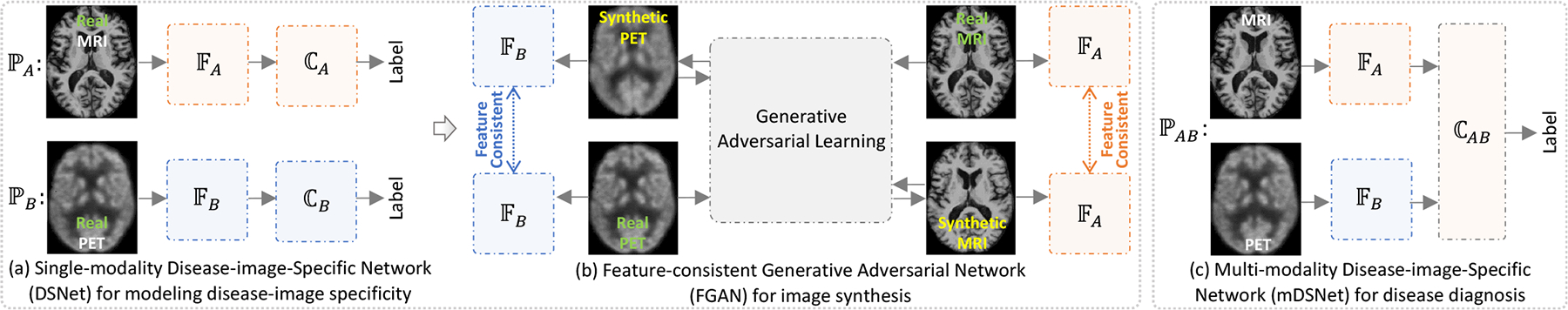
Illustration of our disease-image-specific deep learning (DSDL) framework. Two major components are included: (a) two single-modality Disease-image-Specific Networks (DSNet) for classification and learning disease-image specificity for MRI (i.e., ) and PET (i.e., ), respectively, and (b) a Feature-consistency Generative Adversarial Network (FGAN) for missing image synthesis, encouraging feature maps (e.g., generated by ) of a synthetic image and its real image to be consistent. Note that and in (b) are initialized by those learned in (a) and kept frozen in FGAN. Based on complete (after imputation via FGAN) paired MRI and PET scans, we further develop a multi-modality DSNet (i.e., ) for brain disease identification by concatenating feature maps of MRI and PET (c). In (a) and (c), the backbone feature extractors (e.g., and ) are followed by a spatial cosine module (e.g., , , and ) for classification.
Comparing to our previous works, the contributions of this work are as follows. More detailed information could be seen in Section I of the Supplementary Materials.
We proposed a unified framework called DSDL for joint image synthesis and AD diagnosis using incomplete multi-modality neuroimages. The missing images are imputed in a diagnosis-oriented manner, and hence the synthetic neuroimages are more consistent with real neuroimages from a diagnostic point of view.
We designed a spatial cosine module to model the disease-image specificity in whole-brain MRI/PET scans implicitly and automatically.
We proposed a feature-consistency constraint, which can assist the image synthesis model to preserve the disease-relevant information during modality transformation.
2. Related Work
2.1. Synthesis of Missing Neuroimages
By providing complementary information, multi-modality neuroimaging data have shown to be effective in achieving holistic understanding of the brain and improving automated identification performance of brain disorders [22]. Since subjects may lack a specific imaging modality the missing data problem has been remaining a common challenge in multi-modality-based diagnosis systems.
Rather than estimating the hand-crafted features of missing images, many machine learning techniques have been developed to impute the missing images directly. For problems with multi-modality imaging data, a popular solution is to perform cross-modality estimation, i.e., synthesizing an image of a specific modality based on the corresponding image of another modality. For instance, Huynh et al. [23] proposed to estimate patches of each computerized tomography (CT) image from its corresponding MR image patches using the structured random forest and auto-context model. Jog et al. [24] attempted to transform T1-weighted MR patches to T2-weighted MR patches by training a bagged ensemble of regression trees. Bano et al. [25] designed a cross-modality convolutional neural network (CNN) with a multi-branch architecture operated on various spatial resolution levels for inference between T1-weighted and T2-weighted MRI scans. Li et al. [22] proposed a 3-layer CNN for estimating PET images from MRI scans for data completion.
Generative adversarial networks (GANs) have been developed for image transformation from a source domain/modality to a target domain/modality [26], [27], [28], [29], [30], [31], [32], [33]. A typical GAN [26] consists of two neural networks: (a) a generator trained to synthesize an output that approximates the real data distribution, and (2) a discriminator trained to differentiate between the synthetic and real images. Recently, variants of GAN have been used in synthesizing medical images [4], [34], [35], [36], [37]. Ben et al. [35] combined a fully CNN with a conditional GAN to predict PET from CT images. Yi et al. [36] used GAN to generate missing magnetic resonance angiography images from T1- and T2-weighted MR images. Sun et al. [11] studied the latent variable representations of different modalities and proposed a flow-based generative model for MRI-to-PET image generation. Pan et al. [4] employed CycGAN to predict PET images from MRI scans and achieved good results in brain disease diagnosis using both real and synthetic multi-modality images. Yan et al. [37] added a structure-consistency loss to the original CycGAN and applied it to estimate MRI data from CT data. In general, these GAN-based image synthesis techniques only pose constraints on data distribution, without considering the discriminative capability of synthetic images in a particular task (e.g., neuroimaging-based brain disease diagnosis). Hence, it is desirable to synthesize missing images via GAN in a task-oriented manner.
2.2. Identification of Disease-relevant Brain Regions
Multi-modality neuroimages have been widely used in automated diagnosis of brain disorders, such as AD and MCI. Previous studies have verified that there exits disease-image specificity. For example, AD and MCI are relevant with brain atrophy, especially in specific regions such as hippocampus and amygdala [17], [38], [39]. Zhang et al. [7] combined the volumetric features extracted from 93 regions of interest (ROIs) in both MRI and PET scans and reported that the most discriminative MRI- and PET-based features are from different brain regions. Zhang et al. [8] further studied the volumetric features of PET and MRI and found that the most discriminative brain regions differ in different tasks. Wachinger et al. [19] studied shape asymmetries of neuroanatomical structures across brain regions and found that the subcortical structures in AD is not symmetric, e.g., shape asymmetry in hippocampus, amygdala, caudate and cortex is predictive of disease onset. Cui et al. [39] focused on hippocampus regions and used a 3D densely connected CNN to combine global shape and local visual features of hippocampus to enhance the performance of AD classification. However, these ROI-based methods ignore relative changes in multiple regions, while relying solely on rigid partition of ROI may ignore small or subtle changes caused by diseases.
To tackle this limitation, patch-based methods have been proposed to capture diseased-relevant pathology in a more flexible manner, without using pre-defined ROIs. Liu et al. [40], [41] partitioned each volume into multiple 3D patches and hierarchically combined patch-based features for AD/MCI identification. Suk et al. [9] developed a deep Boltzmann machine to find latent hierarchical feature representation from paired 3D patches of MRI and PET. Based on hand-crafted morphological features, Zhang et al. [42], [43] first defined multiple disease-relevant anatomical landmarks via group-wise comparison, and then extracted features from image patches around these landmarks for automated disease diagnosis. Similarly, Li et al. [44] detected anatomical landmarks and developed a multi-channel CNN for identifying autism spectrum disorder. Liu et al. [21] and Pan et al. [4] proposed deep learning models with multiple sub-networks to learn image-level representations from multiple local patches located by anatomical landmarks. Note that these methods generally rely on hand-crafted features to select disease-relevant locations (via ROIs or anatomical landmarks), Hence, they have to treat patch selection and classifier training as two standalone steps, thus leading to that those selected patches may not well coordinated subsequent classifiers.
Without pre-defining disease-relevant regions and patches, Lian et al. [17] developed a hierarchical fully convolutional network (FCN) to automatically identify discriminative local patches and regions in whole-brain MR images, upon which task-driven MRI features were then jointly learned and fused to construct hierarchical classification models for disease identification. However, this method cannot explicitly reveal the importance of different brain regions, and also cannot be applied to problems with incomplete multi-modality images.
3. Method
3.1. Problem Formulation
We aim to construct a computer-aided diagnosis system based on multi-modality data, such as MRI (denoted as ) and PET (denoted as ) data. Denote as a dataset consisting of N subjects, where and represent, respectively, the MRI scan, PET scan of the ith subject. Also, yi ∈ {0, 1} denotes the class label of the ith subject, e.g., 1 for AD and 0 for cognitively normal (CN) subjects. An automated diagnosis model with multi-modality data can be formulated as
| (1) |
where is the estimated label for the ith subject.
In practice, however, not all subjects have complete data of both modalities. Accordingly, we assume only the first Nc subjects have complete data (i.e., paired MRI and PET scans) and the remaining N − Nc subjects have only one imaging modality (e.g., MRI). The diagnosis model can only be learned based on the first Nc subjects with complete multi-modality data as
| (2) |
where those N − Nc modality-incomplete subjects cannot be used for model learning. Meanwhile, the model defined in Eq. 2 cannot be used to perform prediction for test subjects with only one imaging modality.
To address this issue, one can impute the missing data (i.e., Bi) for the ith subject, by estimating a virtual based on the available modality (i.e., Ai), considering the underlying relevance between two imaging modalities. Denote as the mapping function from MRI to PET, i.e., . Then, the diagnosis model can be executed on modality-incomplete subjects as
| (3) |
Based on modality-complete (after imputation) data, can be learned by using all subjects as
| (4) |
According to Eqs. 3–4, there are two sequential tasks in the automated diagnosis of incomplete multi-modality data, including (1) learning a reliable mapping function for data imputation (i.e., ) to synthesize missing data for modality-incomplete subjects, and (2) learning a classification model (i.e., ) to effectively use multi-modality data for brain disease diagnosis. If these two tasks are performed independently [4], [13], the synthesized data may not be well coordinated with the subsequent diagnosis task. Therefore, we propose the DSDL framework to jointly perform both tasks of image synthesis and disease diagnosis. As illustrated in Fig. 1, this framework include three major components: (1) two single-modality DSNets, i.e., and , for disease diagnosis and learning disease-image specificity; (2) a FGAN for missing image synthesis; and (3) a multi-modality DSNet (i.e., ) for brain disease identification. By jointly training DSNet and FGAN, we can encourage that the disease-image specificity learned by DSNet can be preserved in the image synthesis process, and also those synthetic images are task-oriented for disease diagnosis by focusing on disease-relevant brain regions in each modality.
3.2. Single-modality DSNet
A specific brain disease is often highly relevant with particular regions [17], [18], [19], [21], and disease-relevant regions may differ in MRI and PET scans [7], [8]. To model such disease-image specificity, we propose two single-modality DSNets (see Fig. 2 (a)) for real MRI and real PET scans, respectively. Using both models, we can directly extract features from each input whole-brain image, and identify disease-relevant regions implicitly in each modality. The identified disease-image specificity will be further employed to aid the image synthesis process conducted by FGAN.
Fig. 2.
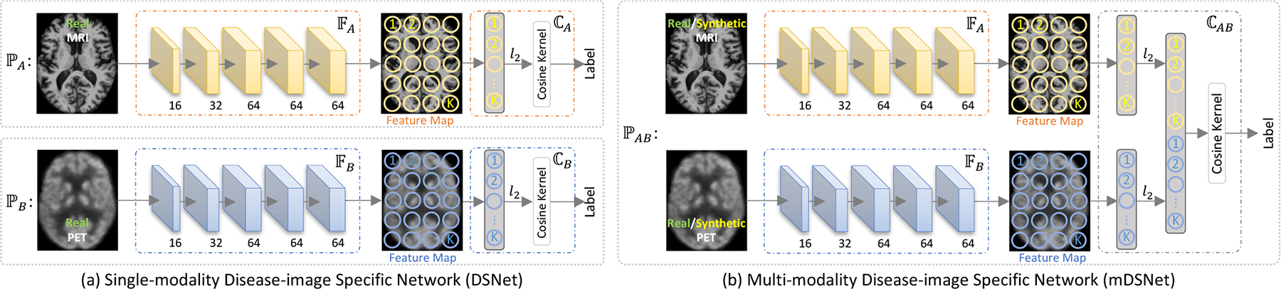
Illustration of the proposed disease-image-specific network (DSNet) for disease classification and modeling disease-image specificity. (a) two single-modality DSNets (i.e., and ) using MRI and PET data, receptively, with each containing a backbone (i.e., or ) for feature extraction and a classifier (i.e., or ) for classification. (b) a multi-modality DSNet (mDSNet) that use paired MRI and PET data as input (i.e., ), with two parallel backbones (i.e., for MRI and for PET) and a classifier (i.e., based on concatenation of features maps generated from two modalities). The backbones (i.e., and ) in single-modality DSNet and mDSNet share the same network architecture but have different input modalities, containing 5 convolutional layers (size: 3 × 3 × 3) with instance normalization and “relu” activation. Also, feature maps of the first 4 convolutional layers are max-pooled, while the feature map of the last layer in each backbone is average-pooled with the stride of 2 × 2 × 2. Here, K denote the elements in the feature map generated by or and K = 4 × 5 × 4 in this work.
3.2.1. Network Architecture
Each single-modality DSNet contains sequentially a backbone feature extraction module (i.e., or ) and a classification module (i.e., or ). The feature extraction module has 5 Conv layers, with 16, 32, 64, 64, and 64 channels, respectively. The first 4 and the last Conv layers are respectively followed by the max-pooling and average-pooling with the stride of 2 and the kernel size of 3 × 3 × 3. For an input image, the feature extraction module outputs its feature maps at each Conv layer. The classification module first l2-normalizes the feature vectors in the feature map of the 5th Conv layer, then concatenates them to construct a spatial representation, and finally uses a fully-connected layer with a spatial cosine kernel to compute the probability score of a subject belonging to a particular category.
3.2.2. Classification with Spatial Cosine Kernel
To facilitate analysis, we decompose each MR/PET image X (X stand for or ) into a disease-relevant part and a residual normal part. After feature extraction by , the output feature map U can be decomposed accordingly into the disease-relevant part Ud and the residual normal part Ur
| (5) |
where α is a coefficient that weighs the relationship between those two parts of a specific subject. Since the residual normal part Ur is not relevant to the disease, the diagnosis result should be independent of it. In other words, the response of the classifier to the entire feature map is only relevant with the disease-relevant part, i.e., .
Since it is difficult to estimate the true value of α for each brain image, we propose a spatial cosine module to suppress the effect of α in DSNet, making the disease-relevant features conspicuous and easy to be captured. Denote U = {v1, v2, ⋯, vK} as the feature map generated by the final Conv layer in a feature extractor, where the kth (k = 1, ⋯, K) element is a vector corresponding to a the kth spatial location in the brain and K = 4 × 5 × 4 is the number of elements in the feature map when input size is 144 × 176 × 144. We first perform l2-normalization on each vector in U, and then concatenate them as the spatial representation of an MRI/PET scan:
| (6) |
through which we can avoid estimating the values of α for different images. Instead of using only the first-order representation in Eq. 6, we further propose the following multiple-order features to represent each input image:
| (7) |
Suppose is a classifier with hyperplane parameters w. With the feature representation of an input scan, is defined as the following spatial cosine kernel
| (8) |
which is equivalent to the product of l2-normalized u and w (both having the constant unit norm). The constant norm forces to focus on the disease-relevant part, since all features have the same norm after l2-normalization (in Eq. 8), and thus suppresses the influence of the residual normal part. More detailed explain of the theory of spatial cosine kernel could be seen in Section 5.4.
3.3. FGAN
Since a pair of MR and PET images scanned from the same subject have underlying relevance but probably different disease-relevant regions, we develop FGAN to synthesize a missing PET image based on its corresponding MRI with a feature-consistency constraint for generating diagnosis-oriented images and an adversarial constraint for generating real-like data. As shown in Fig. 3, our FGAN mainly contains a generative adversarial learning component and two feature-consistency components for MRI and PET modalities, respectively.
Fig. 3.
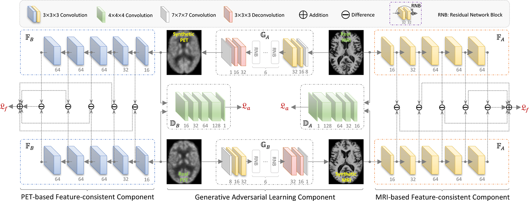
Illustration of our feature-consistency generative adversarial network (FGAN) for image synthesis. It contains (1) two feature-consistency components (i.e., MRI-based and PET-based components) to encourage feature maps of a synthetic image to be consistent with those of its corresponding real image, and (2) a generative adversarial learning component to synthesize images under the constraints of feature consistency (i.e., ) and distribution consistency (i.e., ). Note that and in two feature-consistency components have same architecture but are learned in MRI-based and PET-based DSNet models, respectively, through which the disease-image specificity learned in DSNets will be employed in the image synthesis process, encouraging FGAN to focus on those disease-relevant regions in each modality. Also, the adversarial components, i.e., and ), are used to constrain the synthetic MRI and PET scans follow the same data distribution of those real MRI and PET scans, respectively. Besides, two generators (i.e., and ) are learned to construct bi-directional mappings between two imaging modalities.
3.3.1. Generative Adversarial Learning Component
Using the generative adversarial learning component, we aim to learn an image generator on modality-complete training subjects, and thus can impute the missing PET image for a test subject with only MRI scan via . An inverse mapping is also learned to build the bi-directional mapping between MRI and PET domains. Denote and as two discriminators that can tell whether an input image is real or synthetic, corresponding to the MRI and PET domains, respectively. With two generators (i.e., and ) and two discriminators (i.e., and ), the adversarial loss is defined as
| (9) |
3.3.2. Feature-consistency Component
To employ the disease-image specificity into FGAN, we design the feature-consistency constraint to encourage that the feature maps of a synthetic image should be consistent with feature maps of its corresponding real image. With each feature extractor (e.g., ) containing 5 Conv layers, we denote the feature map of its jth layer as . As shown in the left and right parts of Fig. 3, to encourage features of a synthetic and its respective real images to be consistent at different abstraction levels, we design the feature-consistency constraint for PET and MRI as
| (10) |
through which the disease-image specificity identified by DSNet (based on real MRI/PET data) can be used to constraint FGAN to focus on those modality-specific disease-relevant regions, rather than the whole-brain image. Namely, FGAN is encouraged to generate diagnosis-oriented images by using the feature-consistency constraint components.
Based on the feature-consistency constraint, the proposed feature-consistency loss is defined as
| (11) |
which encourages that a pair of synthetic and real scans from the same modality share the same disease-image specificity.
Finally, the overall loss function of FGAN is defined as
| (12) |
3.3.3. Network Architecture
As shown in Fig. 3, each generator (e.g., ) in our FGAN consists of 3 Conv layers (with 8, 16, and 32 channels, respectively) to extract the knowledge of images in the original domain (e.g., ), 6 residual network blocks (RNBs) [45] to transfer the knowledge from the original domain to the target domain (e.g., ), and 2 deconvolutional (Deconv) layers (with 32 and 16 channels, respectively) and 1 Conv layer (with 1 channel) to construct the image in the target domain. Each discriminator (e.g., ) contains 5 Conv layers, with 16, 32, 64, 128, and 1 channel(s), respectively. It outputs an indicator to tell whether the input pair of real image (e.g., B) and synthetic image (e.g., ) are distinguishable (output: 0) or not (output: 1). Besides, each feature-consistency component contains two parallel subnetworks (e.g., ) that share the same architecture and parameters with the feature extractor in each modality in our DSNet (e.g., ). Note that and in Fig. 1 (b) are initialized by those learned in Fig. 1 (a) and kept frozen in FGAN. It inputs a pair of real image (e.g., ) and synthetic image (e.g., ), and outputs a differential score to indicate the similarity between the feature maps of the real and its corresponding synthetic image. Hence, the disease-image specificity learned in DSNet can be used to aid the image imputation process in FGAN, i.e., the modality-specific disease-relevant regions will be more effectively synthesized in a diagnosis-oriented manner. In turn, synthetic images could be more relevant to the task of brain disease diagnosis, thus boosting the learning performance.
3.3.4. Model Extension
Besides the loss function defined in Eq. 12, we further extend our FGAN model by using several additional constraints, such as the voxel-wise-consistency constraint [28] and cycle-consistency constraint [4], [32]. In this work, we denote the FGAN with an additional voxel-wise-consistency constraint as FVoxGAN, and denote the FGAN with an addition cycle-consistency constraint as FCycGAN. Specifically, the corresponding losses of FVoxGAN and FCycGAN are defined, respectively, as
| (13) |
and
| (14) |
where the voxel-wise-consistency loss in Eq. 13 and cycle-consistency loss in Eq. 14 are defined, respectively, as
| (15) |
and
| (16) |
Different from the adversarial loss and feature-consistency loss that rely on specific sub-networks, the voxel-wise-consistency loss in FVoxGAN and cycle-consistency loss in FCycGAN can be directly apply to paired real and synthetic images. Therefore, our FGAN and its two extensions share the same network architecture (see Fig. 3) but have different loss functions.
3.4. Multi-modality DSNet
Using the proposed FGAN, one can obtain synthetic MRI/PET scans for modality-incomplete subjects, and thus each subject will be represented by complete multi-modality data (i.e., a pair of MRI and PET scans). To handle classification problems with multi-modality data, we extend our single-modality DSNet to a multi-modality version, called mDSNet.
As shown in Fig. 2 (b), our mDSNet consists of sequentially two parts: (1) two parallel feature extraction modules (i.e., and ) followed by a feature map concatenation operation to fuse futures of MRI and PET and (2) a classifier (i.e., ) with the multi-order feature representation (see Eq. 7) as its input. The feature extraction modules in mDSNet have the same network architecture as DSNet but different parameters. The proposed mDSNet is trained from sketch using both the real and synthetic images. Since the classifier can also input the first-order feature representation (see Eq. 6), we denote mDSNet with first-order features as mDSNet-1st in this work.
3.5. Implementation Details
In the training stage, the proposed DSDL framework is executed via the following three stages: (1) using only the real MRI (i.e., ) and real PET (i.e., ) data to train two single-modality DSNets (i.e., and ), respectively, for Disease-image Specificity Identification; (2) using modality-complete subjects with real MRI and PET data to train FGAN for image synthesis; and (3) using the complete (after imputation) paired MRI and PET scans of all training subjects to train mDSNet for disease diagnosis. Note that, to augment the number of samples, The combination (Ai, ) will also be used as a training sample to train mDSNet even Bi exists.
In the test stage, for an unseen test subject with complete multi-modality data, we directly feed its MRI and PET scans to mDSNet for classification. Given an unseen test subject with missing MRI/PET scan, we first impute the missing scan using our trained FGAN model and then feed the complete (after imputation) paired MRI and PET scans into mDSNet for classification.
Our proposed models are implemented by Python with Tensorflow on a platform with GTX 1080 Ti and Intel Core i7-8700. We first train two DSNets and for 40 epochs using complete subjects (i.e., those with paired PET and MR images). We then train and by minimizing with fixed and , and train and by minimizing with fixed and , iteratively, for 100 epochs. After that, we train mDSNet for 40 epochs using both real and synthetic data. We use SGD solver with a learning rate 1 × 10⁻³ to train DSNets and mDSNet, and use the Adam solver [46] with a learning rate of 2 × 10⁻³ to train FGAN. The batch size is set to 1 due to the limitation of GPU memory. More details on hyper-parameter settings could be seen in the Supplementary Materials.
4. Experiments
4.1. Materials and Image Pre-processing
We first evaluated the proposed method on two subsets of ADNI [5], including ADNI-1 and ADNI-2. Subjects in these two datasets were divided into four categories: (1) AD, (2) CN, (3) progressive MCI (pMCI) that would progress to AD within 36 months after baseline, and (4) static MCI (sMCI) that would not progress to AD. After removing these subjects appearing in both ADNI-1 and ADNI-2 from ADNI-2, there are 205 AD, 231 CN, 165 pMCI and 147 sMCI subjects in ADNI-1, while there are 162 AD, 209 CN, 89 pMCI and 256 sMCI subjects in ADNI-2. All the above subjects in ADNI-1 and ADNI-2 have baseline MRI data, while only 356 and 581 of these subjects have PET images in ADNI-1 and ADNI-2, respectively. We also used the AIBL [47] dataset for performance evaluation, containing 71 AD and 447 CN subjects. Similar to ADNI-1 and ADNI-2, all subjects in AIBL have MRI scans, and only part of them have PET scans. The demographic and clinical information of three datasets are listed in Table 1. More details of these data are described in Section 2 of the Supplementary Materials.
TABLE 1.
The demographic and clinical information of studied subjects with four categories (Cat.) from three datasets. The education (Edu.) years and the mini-mental state examination (MMSE) values are reported in terms of mean ± standard deviation. M: Male; F: Female.
| Dataset | Cat. | MRI/PET | M/F | Age | Edu. | MMSE |
|---|---|---|---|---|---|---|
| ADNI-1 | AD | 205/95 | 106/99 | 76 ± 8 | 14 ± 4 | 23 ± 2 |
| CN | 231/102 | 119/112 | 76 ± 5 | 16 ± 3 | 29 ± 1 | |
| pMCI | 165/76 | 100/65 | 75 ± 7 | 16 ± 3 | 27 ± 2 | |
| sMCI | 147/83 | 101/46 | 75 ± 8 | 16 ± 4 | 27 ± 2 | |
| ADNI-2 | AD | 162/142 | 95/70 | 75 ± 8 | 16 ± 3 | 23 ± 3 |
| CN | 209/186 | 99/110 | 73 ± 6 | 16 ± 3 | 27 ± 2 | |
| pMCI | 89/80 | 52/37 | 73 ± 7 | 16 ± 3 | 28 ± 2 | |
| sMCI | 256/173 | 146/110 | 71 ± 8 | 16 ± 3 | 27 ± 2 | |
| AIBL | AD | 71/62 | 30/41 | 73 ± 8 | – | 27 ± 4 |
| CN | 447/407 | 192/254 | 72 ± 7 | – | 28 ± 4 |
For data pre-processing, we first performed skull-stripping on MRI scans using FreeSurfer [48], and then linearly aligned each PET scan to its corresponding MRI scan. Next, we affine each MRI scan to the commonly-used MNI template using SPM [49], while its corresponding PET scan (if existed) is also affined using the same affination parameter. In this way, each pair of MRI and PET scans of a same subject have the spatial correspondence.
We performed two groups of experiments on the ADNI-1 and ADNI-2 datasets: synthesizing MR and PET images and diagnosing brain diseases, including AD identification (AD vs. CN classification) and MCI conversion prediction (pMCI vs. sMCI classification). To evaluate the generalization capability of our proposed models for image synthesis and disease classification, we further performed an extra group of experiments on the AIBL dataset.
4.2. Evaluation of Synthetic Neuroimages
4.2.1. Competing Methods
We first evaluate the quality of synthetic images generated by three typical GANs, including (1) conventional GAN with only an adversarial loss, (2) cycle-consistency GAN (CycGAN) [4], [32] with an additional cycle-consistency constraint, and (3) GAN with a voxel-wise-consistency constraint (VoxGAN) [28], our FGAN, and its two variants, i.e., FVoxGAN and FCycGAN. For the fair comparison, FGAN and its variants share the same network architecture as shown in Fig. 3 but have different losses. The other three GANs have the same architecture as the generative adversarial learning component of FGAN (the middle part of Fig. 3) but different losses.
4.2.2. Experimental Setup
We trained six GANs using the subjects with real MRI and PET scans in ADNI-1, and tested the trained models on complete subjects (with both real MRI and real PET scans) in ADNI-2. We used four metrics to measure the quality of synthetic images, including (1) the mean absolute error (MAE), (2) the mean square error (MSE), (3) peak signal-to-noise ratio (PSNR), and (4) structural similarity index measure (SSIM) [50].
To evaluate the reliability of synthetic MR and PET images in disease diagnosis, we further reported the values of the area under receiver operating characteristic (AUC) achieved by our single-modality DSNet model on both AD identification (denoted as AUC*) and MCI conversion prediction (denoted as AUC†). We first trained MRI- and PET-based DSNet models on complete subjects (i.e., with both real MRI and real PET scans) in ADNI-1, respectively, and then applied these two DSNets to subjects in ADNI-2 represented by synthetic MR and PET images, respectively, for classification.
4.2.3. Results of Image Synthesis
In Table 2, we report the results achieved by six different methods in synthesizing MRI and PET scans. Four interesting observations can be found from Table 2. First, five advanced GAN methods (i.e., CycGAN, VoxGAN, FCycGAN, FVoxGAN, and FGAN) generally yield better results than the baseline GAN. This implies that the cycle-consistency loss, voxel-wise-consistency loss, and feature-consistency loss are positive constraints to help synthesize images with higher quality, in terms of both image similarity and discrimination in subsequent diagnosis tasks. It verifies that spatial structure information is useful for computer-aided AD diagnosis. Second, The AUC values obtained by using synthetic images generated by our FGAN-based methods (i.e., FGAN, FCycGAN, and FVoxGAN) are significantly higher than those using synthetic images generated by three competing methods (i.e., GAN, CycGAN, and VoxGAN) in both classification tasks. The possible reason is that the proposed feature-consistency constraint is effective to encourage GAN models to generate diagnosis-oriented images (rather than focusing on whole-brain regions), thus helping boost the performance of brain disease diagnosis. Besides, regarding four metrics for image quality (i.e., MAE, MSE, SSIM and PSNR), our FGAN models consistently outperforms CycGAN and GAN in synthesizing both MRI and PET scans, but only achieves comparable results compared with VoxGAN. This implies that the proposed feature-consistency loss is a strong constraint to encourage good quality of synthetic images, but not as strong as the voxel-wise-consistency loss used in VoxGAN. However, using the voxel-wise-consistency loss and feature-consistency loss simultaneously (as we do in FVoxGAN) does not significantly improve the quality of synthetic images. It implies that the feature-consistency loss and voxel-wise-consistency loss may have potential competitive relationships. Furthermore, the AUC values (i.e. AUC* and AUC†) achieved by six methods based on synthetic PET data are observably lower than based on synthetic MRI, which indicates it may be more hard to synthesize classifiable PET from MRI than synthesize MRI from PET. The possible reason is that PET scans contain comparable structure information with MRI while MRI contain insufficient functional information to be passed to synthetic PET.
TABLE 2.
Results(% except PSNR) of image synthesis achieved by six different methods for MRI and PET scans of subjects in ADNI-2, with the models trained on ADNI-1.
| Method | Synthetic MRI | Synthetic PET | ||||||||||
|---|---|---|---|---|---|---|---|---|---|---|---|---|
| MAE | MSE | SSIM | PSNR | AUC* | AUC† | MAE | MSE | SSIM | PSNR | AUC* | AUC† | |
| GAN | 10.66 | 3.68 | 59.34 | 26.43 | 66.69 | 52.86 | 10.79 | 3.05 | 57.41 | 27.27 | 52.92 | 51.54 |
| ±0.77 | ±0.54 | ±2.78 | ±0.59 | ±1.00 | ±0.63 | ±2.82 | ±0.77 | |||||
| CycGAN | 10.16 | 3.33 | 60.55 | 26.86 | 82.35 | 65.68 | 10.36 | 2.53 | 57.41 | 27.56 | 57.50 | 52.55 |
| ±0.78 | ±0.51 | ±3.06 | ±0.65 | ±1.25 | ±0.69 | ±3.54 | ±0.96 | |||||
| VoxGAN | 8.10 | 2.17 | 69.74 | 28.75 | 88.12 | 66.85 | 7.61 | 1.55 | 70.23 | 30.40 | 82.66 | 68.65 |
| ±0.81 | ±0.46 | ±3.95 | ±0.79 | ±1.42 | ±0.62 | ±5.48 | ±1.48 | |||||
| FGAN (Ours) | 8.64 | 2.27 | 68.20 | 28.56 | 94.06 | 78.05 | 8.24 | 1.80 | 67.34 | 29.70 | 86.05 | 70.63 |
| ±0.83 | ±0.47 | ±3.65 | ±0.78 | ±1.37 | ±0.63 | ±4.97 | ±1.29 | |||||
| FCycGAN (Ours) | 8.69 | 2.39 | 67.20 | 28.34 | 93.22 | 78.92 | 8.54 | 1.94 | 65.85 | 29.38 | 86.10 | 69.24 |
| ±0.87 | ±0.51 | ±3.52 | ±0.81 | ±1.51 | ±0.69 | ±5.21 | ±1.36 | |||||
| FVoxGAN (Ours) | 8.38 | 2.26 | 68.25 | 28.59 | 93.23 | 78.45 | 8.42 | 1.89 | 66.16 | 29.48 | 86.10 | 72.22 |
| ±0.87 | ±0.52 | ±3.63 | ±0.81 | ±1.37 | ±0.64 | ±4.92 | ±1.27 | |||||
Fig. 4 visualizes the ground truth MR and PET images of a CN subject (Roster ID: 4386) and an AD subject (Roster ID: 4997) in ADNI-2 and the synthetic images generated by GAN, cycGAN (used in our previous work), VoxGAN, and our FGAN, respectively. To show sufficient details, the region in the pink / green rectangular on each image was enlarged and displayed to the right of the image. It reveals that the images synthesized by our FGAN (4th column) are more consistent with the ground truth (5th column) than those synthesized by other GANs (1st-3rd columns), particularly in terms of the ventricle size and sulcus width. It can be attributed to the fact that, comparing to the voxel-consistency constraint and cycle-consistency constraint, the feature-consistency constraint used in FGAN is a high-level constraint, which can encourage pattern similarities rather than only voxel-level similarities. More views and more examples and supplied in Figs. S3–S5 of the Supplementary Materials.
Fig. 4.
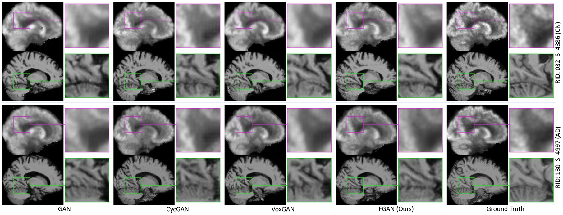
PET and MRI scans synthesized by four methods for two typical subjects (Roster IDs: 4386, 4997) in ADNI-2, along with their corresponding ground-truth images. All six image synthesis models are trained on ADNI-1.
4.3. Evaluation of Automated Diseases Diagnosis
4.3.1. Competing Methods
We further evaluated our mDSNet on both tasks of AD identification and MCI conversion prediction against two conventional methods using concatenated MRI and PET features, i.e., (1) ROI method [7], [51], and (2) patch-based morphology (PBM) [9], [52] and two deep learning models, i.e., (3) landmark-based deep multi-instance learning (LDMIL) method [21], and (4) a conventional CNN method. For ROI, PBM and LDMIL methods, we used default parameter settings in their original papers. For the fair comparison, the CNN method shares the similar network architecture with our mDSNet (see Fig. 2 (b)) but a different classification module. That is, CNN globally averages the feature map of the last Conv layer and uses a fully connected layer for classification (instead of using the spatial cosine module in mDSNet). To investigate the effect of multi-order representation in Eq. 7, we compare the mDSNet-1st that use first-order features defined in Eq. 6.
4.3.2. Experimental Setup
These classification methods utilize all subjects with both real multi-modality scans and synthetic PET images generated by our FGAN. We also performed experiments on complete subjects (with real paired MRI and PET scans), and denoted the corresponding methods as “-C”. Since all subjects have MRI scans in ADNI-1 and ADNI-2 datasets, we also reported the results of different methods using only MRI modality, and denoted the corresponding methods as “-M”. For all methods, classifiers are trained on ADNI-1, and tested on the independent ADNI-2 and AIBL datasets, respectively. We employ six metrics for performance evaluation in disease diagnosis, including (1) AUC, (2) accuracy (ACC), (3) sensitivity (SEN), (4) specificity (SPE), (5) F1-Score (F1S), and (6) Matthews correlation coefficient (MCC) [53].
4.3.3. Disease Identification Results on ADNI-2
With models trained on ADNI-1, the disease classification results achieved by different methods on ADNI-2 are reported in Table 3. From Table 3, we can see that our mDSNet generally achieves the best performance in most cases. For instance, using both real and synthetic images, our mDSNet method achieves the highest AUC values (97.23%, 84.44%) in the tasks of AD vs. CN and pMCI vs. sMCI classification. This suggests that our mDSNet is reliable in automated AD diagnosis and progression prediction of MCI patients, which is potentially very useful in practice. Besides, our mDSNet yields slightly better results compared to LDMIL that pre-defines disease-relevant regions in brain images via anatomical landmarks [54]. This implies that the proposed spatial cosine kernel provides an efficient strategy to capture the disease-image specificity embedded in neuroimages. On the other hand, methods (e.g., mDSNet) using all subjects with complete multi-modality data (after imputation via FGAN) consistently outperform their counterparts (e.g., mDSNet-C) that utilize modality-complete subjects with real MRI and PET scans, and are superior to their counterparts (e.g., mDSNet-M) using all subjects with real MRI scans. For example, mDSNet achieves an MCC value of 52.47 in MCI conversion prediction, which is higher than the results of mDSNet-C (46.52) and mDSNet-M (51.27). The possible reason could be that, compared with mDSNet-C, more subjects are used for model training in mDSNet. Even though mDSet-M (using only real MRI data) and mDSNet used the same number of training subjects, mDSNet takes advantage of data from an additional imaging modality (i.e., real and synthetic PET images). These results demonstrate that neuroimages generated by our FGAN model are useful in promoting the diagnostic performance.
TABLE 3.
Diagnosis results (%) achieved by six different methods, with classification models trained on ADNI-1 and tested on ADNI2. Methods marked as “-M” denote that only subjects with real MRI scans are used for model training, methods marked as “-C” denote that modality-complete subjects (with real paired MRI and PET scans) are used for model training, while the remaining methods employ all subjects (with both real images and synthetic PET images generated by FGAN) in two classification tasks.
| Method | AD vs. CN Classification | pMCI vs. sMCI Classification | ||||||||||
|---|---|---|---|---|---|---|---|---|---|---|---|---|
| AUC | ACC | SPE | SEN | F1S | MCC | AUC | ACC | SPE | SEN | F1S | MCC | |
| ROI-M | 86.22 | 79.41 | 83.64 | 76.08 | 78.19 | 59.30 | 70.48 | 66.38 | 62.92 | 67.58 | 49.12 | 27.21 |
| PBM-M | 88.11 | 82.22 | 77.36 | 86.07 | 79.35 | 63.83 | 73.21 | 68.70 | 58.43 | 72.27 | 49.06 | 28.04 |
| LDMIL-M | 95.77 | 90.37 | 88.48 | 91.87 | 89.02 | 80.46 | 80.35 | 73.33 | 73.03 | 73.44 | 58.56 | 41.77 |
| CNN-M | 93.87 | 88.24 | 87.27 | 89.00 | 86.75 | 76.18 | 76.59 | 72.46 | 66.29 | 74.61 | 55.40 | 37.29 |
| mDSNet-1st-M (Ours) | 95.68 | 90.11 | 89.70 | 90.43 | 88.89 | 79.99 | 82.36 | 75.65 | 73.03 | 76.56 | 60.75 | 45.14 |
| mDSNet-M (Ours) | 96.31 | 90.64 | 89.70 | 91.39 | 89.42 | 81.03 | 81.84 | 76.23 | 74.16 | 76.95 | 61.68 | 46.52 |
| ROI-C | 88.95 | 81.49 | 82.99 | 80.32 | 79.74 | 62.92 | 69.17 | 66.92 | 42.50 | 77.78 | 44.16 | 20.74 |
| PBM-C | 87.87 | 82.39 | 80.27 | 84.04 | 80.00 | 64.27 | 68.04 | 68.85 | 60.00 | 72.78 | 54.24 | 31.28 |
| LDMIL-C | 95.64 | 90.75 | 88.44 | 92.55 | 89.35 | 81.18 | 82.62 | 76.92 | 71.25 | 79.44 | 65.52 | 48.67 |
| CNN-C | 94.40 | 89.25 | 88.44 | 89.89 | 87.84 | 78.22 | 78.70 | 75.00 | 67.50 | 78.33 | 62.43 | 44.13 |
| mDSNet-1st-C (Ours) | 95.78 | 90.45 | 89.80 | 90.96 | 89.19 | 80.64 | 82.74 | 76.15 | 76.25 | 76.11 | 66.30 | 49.33 |
| mDSNet-C (Ours) | 96.26 | 91.46 | 90.85 | 91.94 | 90.21 | 82.65 | 83.06 | 77.47 | 75.00 | 78.61 | 67.80 | 51.27 |
| ROI | 90.51 | 83.42 | 84.24 | 82.78 | 81.76 | 66.69 | 72.31 | 71.30 | 52.81 | 77.73 | 48.70 | 29.12 |
| PBM | 91.46 | 84.49 | 81.21 | 87.08 | 82.21 | 68.48 | 72.79 | 71.88 | 64.04 | 74.61 | 54.03 | 35.37 |
| LDMIL | 96.76 | 91.71 | 88.48 | 94.26 | 90.40 | 83.17 | 83.89 | 79.71 | 71.91 | 82.42 | 64.65 | 51.13 |
| CNN | 94.72 | 89.57 | 85.45 | 92.82 | 87.85 | 78.82 | 79.98 | 76.52 | 69.66 | 78.91 | 60.49 | 44.98 |
| mDSNet-1st (Ours) | 97.02 | 92.25 | 90.91 | 93.30 | 91.18 | 84.27 | 83.94 | 80.00 | 70.79 | 83.20 | 64.61 | 51.20 |
| mDSNet (Ours) | 97.23 | 93.05 | 90.91 | 94.74 | 92.02 | 85.88 | 84.44 | 79.71 | 75.28 | 81.25 | 65.69 | 52.47 |
4.3.4. Disease Identification Results on AIBL
We further use AIBL as the testing set for classification performance evaluation. Different from the ADNI, we only use synthesized PET in AIBL for testing to simulate the case that all subjects refused PET scanning. For the fair comparison, six methods utilize all subjects with real MRI scans and synthetic PET scans (generated by FGAN). Results of different methods in AD vs. CN classification are reported in Table 4, considering that AIBL contains a limited number of MCI subjects.
TABLE 4.
Diagnosis results (%) achieved by six different methods using all subjects with only real MRI scans (denoted as “-M”) and with both real MRI images and synthetic PET images (generated by FGAN) in AC vs. CN. classification. Classification models are trained on ADNI-1 and tested on AIBL.
| Method | AD vs. CN Classification | |||||
|---|---|---|---|---|---|---|
| AUC | ACC | SPE | SEN | F1S | MCC | |
| ROI-M | 83.49 | 73.69 | 76.06 | 73.32 | 44.26 | 36.02 |
| PBM-M | 86.34 | 78.34 | 80.28 | 78.03 | 50.44 | 43.80 |
| LDMIL-M | 93.81 | 87.64 | 87.32 | 87.70 | 65.96 | 61.70 |
| CNN-M | 91.23 | 83.78 | 83.09 | 83.89 | 58.41 | 53.00 |
| DSNet-1st-M (Ours) | 93.98 | 88.80 | 85.92 | 89.26 | 67.78 | 63.43 |
| DSNet-M (Ours) | 94.39 | 89.77 | 83.10 | 90.83 | 69.01 | 64.41 |
| ROI | 87.25 | 79.69 | 85.92 | 78.70 | 53.74 | 48.45 |
| PBM | 90.63 | 80.66 | 85.92 | 79.82 | 54.95 | 49.76 |
| LDMIL | 93.64 | 88.03 | 87.32 | 88.14 | 66.67 | 62.45 |
| GANN | 92.77 | 88.42 | 84.51 | 89.04 | 66.67 | 62.05 |
| mDSNet-1st (Ours) | 94.37 | 89.77 | 87.32 | 90.16 | 70.06 | 66.05 |
| mDSNet (Ours) | 94.92 | 90.35 | 87.32 | 90.83 | 71.26 | 67.34 |
From Table 4, we can see that four deep learning methods (i.e., LDMIL, CNN, mDSNet-1st, and mDSNet) generally outperform two conventional approaches (i.e., ROI and PBM) that use hand-crafted imaging features. This suggests that integrating feature extraction and classifier construction into a unified framework can boost the diagnosis performance. Besides, mDSNet based on multi-order representation usually outperforms mDSNet-1st (using first-order features) and CNN (using average-pooling-based features). This implies that using both first-order and second-order features in our mDSNet is more efficient in capturing the disease-image specificity embedded in neuroimages, compared with using only first-order representation and average pooling based features.
5. Discussion
5.1. Effect of Feature Maps
In the feature-consistency component (Fig. 3), we add the feature-consistency constraint at each of five Conv layers. To investigate the effect of our feature-consistency constraint at different layers, we perform an experiment by adding such a constraint at only one single Conv layer, and denote the generated FGAN variants as . Based on the resulting FGAN models, we can obtain synthetic MRI and PET images. The image quality of these images (regarding SSIM and PSNR) and their performance in AD vs. CN classification (with AUC values marked as *) and pMCI vs. sMCI classification (with AUC values marked as †) are shown in Fig. 5. Fig. 5 reveals that adding the feature-consistency constraint on early layers (e.g., l1) generally results in better synthesis results (in term of SSIM and PSNR) but lower classification results (in term of AUCs). Also, models using such a constraint at the late layers (e.g. l5) usually generate the reverse results (i.e., better classification performance but low image quality). Therefore, we add the feature-consistency constraint to feature maps of all five Conv layers to balance the synthesis results and classification results.
Fig. 5.
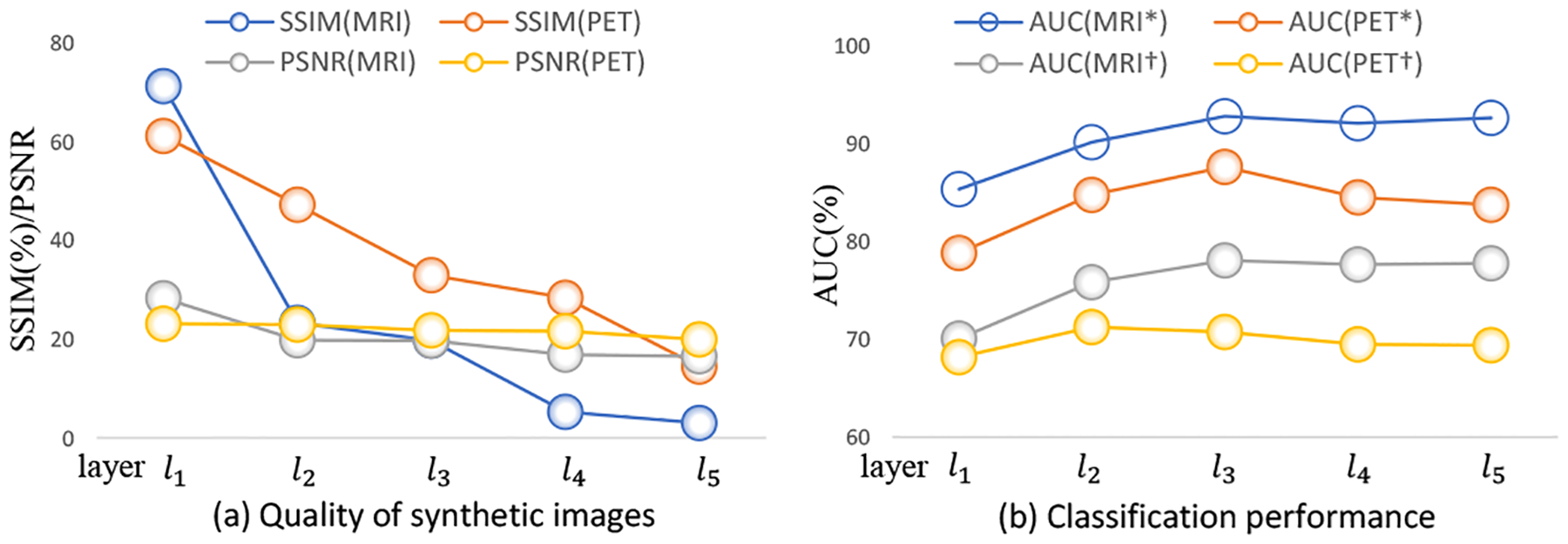
Quality (a) and classification performance (b) of synthetic images generated by five FGAN variants using the feature-consistency constraint on feature maps at only one single Conv layer (e.g., the i-th layer li) in and .
5.2. Comparison of Different Losses
To evaluate the influence of different losses used in our image synthesis models (i.e., FGAN, FCycGAN and FVoxGAN), we further train the generative model (with only and in Fig. 3) with only one of the following losses: (1) adversarial loss , (2) cycle-consistency loss , (3) voxel-wise-consistency loss , and (4) feature-consistency loss . Using each of four different losses, the corresponding generative model can generate synthetic MRI and PET scans. In Fig. 6 (a)–(b), we show the resulting MAE values of these synthetic image along the training epochs. Based on these generated images, we further report the AUC values of our mDSNet in AD vs. CN classification in Fig. 6 (c)–(d), with models trained on ADNI-1 and tested on ADNI-2. Fig. 6 (a)–(b) suggests, when using four different losses, the model that uses only the voxel-wise-consistency loss can produce the most visually realistic image (with respect to MAE values). From Fig. 6 (c)–(d), one can observe that the model using the feature-consistency loss consistently achieves the best classification performance (regarding AUC values), compared with those using the other three losses. Meanwhile, models with the voxel-wise-consistency loss and our feature-consistency loss are more stable compared to those with cycle-consistency loss and adversarial loss. This could be due to the fact that the calculation of the latter two losses relies on updating modules, i.e., another generator and discriminator.
Fig. 6.
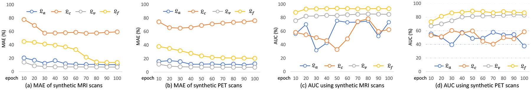
Performance of the generative component of FGAN in image synthesis versus the numbers of training epochs. The model was trained on ADNI-1 with only single loss and tested on ADNI-2. Four loss functions were evaluated, including the adversarial loss , cycle-consistency loss , voxel-wise-consistency loss , and feature-consistency loss .
5.3. Enhancing Diagnosis Performance by More Subjects
In the previous experiments, we only use these subjects in ADNI-1 to train our diagnosis model. Since more data may result in better performance, it is possible to use more subjects (e.g., those from ADNI-2) to further improve the performance of the diagnosis performance. Accordingly, we perform another experiment by using both the images in ADNI-1 and ADNI-2 to train the diagnosis model (i.e., mDSNet) but using only complete subjects in ADNI-1 to train the FGAN model. Then we apply the obtained models on the AIBL dataset, with results (denoted as mDSNet-2) reported in Table 5 as well as the original results (denoted by mDSNet). It seems this strategy slightly improves the diagnosis performance (e.g. the AUC score increases from 94.92% to 95.31%). The possible reason could be that more training data make the learned model more general among different sites, thus improving the diagnosis performance.
TABLE 5.
Comparison of our mDSNet on AIBL while using only ADNI-1 or using both ADNI-1 and ADNI-2 for training in stage (3).
| Method | AD vs. CN Classification | |||||
|---|---|---|---|---|---|---|
| AUC | ACC | SPE | SEN | F1S | MCC | |
| mDSNet | 94.92 | 90.35 | 87.32 | 90.83 | 71.26 | 67.34 |
| mDSNet-2 | 95.31 | 90.73 | 88.73 | 91.05 | 72.41 | 68.74 |
5.4. More Details of Spatial Cosine Kernel
Following the description of spatial cosine kernel in section 3.2.2, the input of our DSNet is a neuroimage of size 144 × 176 × 144 and the l2-normalized feature map (spatial representation) is denoted as u = (u1, u2, ⋯, uK) where . The spatial cosine kernel (defined in Eq. 8) is
| (17) |
where w is the ensemble of hyper-parameters. Due to having the same dimension as u, w can be partitioned into K elements, i.e., w = (w1, w2, ⋯, wK), where wk has same dimension as uk. Let , , then the spatial cosine kernel can be rewritten as accumulating the similarity between wk and the k-th element in a feature map as
| (18) |
Herein, is a cosine kernel that indicates the group difference corresponding to the k-th elements. Meanwhile, βk, directly proportional to the norm of wk, indicates the contribution coefficient of the k-th cosine kernel to the classification result. Since βk is learned automatically and implicitly while training DSNet, it is very convenient to capture the disease-relevant patterns by finding the disease-relevant part of the feature map (Ud), in which each uk corresponds to a large βk.
Furthermore, it should be noted that the disease-relevant part (Ud), the residual normal part (Ur), and α are mutually dependent but only one constraint in Eq. 5 should be satisfied. Hence, the decomposition of disease-relevant part and residual normal part is not unique. For example, a possible decomposition of a feature map U could be
| (19) |
where the disease-relevant component of each pattern is placed to the disease-relevant part, and the disease-irrelevant component of each pattern is placed to the residual normal part. In this case, .
Alternatively, we can use a threshold τ to binarize βk as follows
| (20) |
and thus decompose U as
| (21) |
It means that we directly place the disease-relevant patterns to disease-relevant parts and place the disease-irrelevant patterns to residual normal part. In this case, . When considering only the prediction labels, we have
| (22) |
Namely, if the disease-relevant parts and residual normal parts can be separated, the coefficient α will not affect the predicted labels.
5.5. Statistical Significance Analysis
The major hypothesis in this work is that a generative model with the feature-consistency constraint can generate the synthetic images which are diagnostically similar to real images. It means that the synthetic images and corresponding real images can deliver similar diagnosis of medical conditions. To verify this, we calculated the inter-class averaged dissimilarity (ICAD) of 80 brain regions in synthetic MRI and PET images and displayed them in Fig. 7. The definition of ICAD is as follows.
Fig. 7.
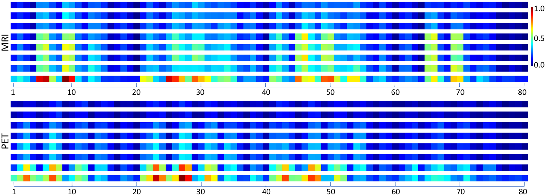
The inter-class averaged dissimilarities (ICAD) and rescaled contribution coefficients of 80 brain region in synthetic MRI and PET images. For each modality, the top six rows are the ICAD of the synthesized images generated by GAN, cycGAN, voxGAN, FGAN, FcycGAN, and FvoxGAN, respectively, the 7th row is the ICAD of real images, and the 8th row is the rescaled value of contribution coefficient. It shows that the disease-relevant regions are different across two modalities.
Suppose the i-th (i ∈ {1, 2, ⋯, N}) scan has a feature map ui = (u1,i, u2,i, ⋯, uK,i)(∥uk,i∥2 = 1) and a class label yi ∈ {0, 1}. The similarity of two feature maps ui and uj is measured by the spatial cosine kernel,
| (23) |
Then, the ICAD, denoted by S, can be calculated as
| (24) |
A large ICAD value indicates that two classes are easy to be distinguished. Similarly, we can use
| (25) |
to measure the distinguishability regarding the k-th location.
For each modality in Fig. 7, the top six rows (denoted as S1, S2, ⋯, S6 from top to bottom) are the ICAD of the synthetic images generated by GAN, cycGAN, voxGAN, FGAN, FcycGAN, and FvoxGAN, respectively, and the 7th row (denoted as S7) is the ICAD of real images. The bottom row for each modality depicts the values of {βk}, which have been rescaled to [0, 1], indicating the contribution coefficient of each region to the classification task. Where, a larger value means that the region is more relevant to the classification task. Comparing the 7th row and the bottom row, it suggests that most of the regions with higher inter-class dissimilarities are recognized as more relevant to disease diagnosis. Meanwhile, it reveals that most disease-relevant regions are different across two modalities, which renders the cross-modality image synthesis a challenging task and also makes the feature-consistency constraint a must for any solutions to this task.
We now conduct the statistical significance analysis for our major hypothesis. The null hypotheses (H0), alternative hypotheses (H1), and the p-values of H0 for MRI and for PET are listed in Table 6. It shows that all obtained p-values are smaller than 0.05. Therefore, H1 is accepted,, which means that a generative model with the feature-consistency constraint can generate images more diagnostically similar to real images.
TABLE 6.
Hypotheses and obtained p-values in our statistical significance analysis.
| Index | Hypotheses H0 | Hypotheses H1 | p-values (MRI) | p-values (PET) |
|---|---|---|---|---|
| 1 | (S1 – S7)2 <= (S4 – S7)2 | (S1 – S7)2 > (S4 – S7)2 | 1.64 × 10⁻⁴ | 7.63 × 10⁻¹¹ |
| 2 | (S2 – S7)2 <= (S5 – S7)2 | (S2 – S7)2 > (S5 – S7)2 | 4.95 × 10⁻⁶ | 9.92 × 10⁻¹¹ |
| 3 | (S3 – S7)2 <= (S6 – S7)2 | (S3 – S7)2 > (S6 – S7)2 | 9.10 × 10⁻⁷ | 1.00 × 10⁻⁶ |
5.6. “Hallucination” in Generative Unseen Patterns
Currently, it is arguable to first train a generative model on available data for absent data generation and then to use the generated data, together with the available data, to train another model for classification. Especially, the generated data may be affected by the dataset used to train the generative model. For example, if each training image contains a tumor, the data generated by the trained model may also contain a tumor, although it is expected to generate the scan of a normal control. On the other hand, if each training data was acquired from a normal control, it is less impossible for the trained generative model to generate a scan with tumors.
In this study, the abovementioned “hallucination” issue must be addressed when we attempt to use cross-modality image generation to impute missing PET data for the multi-modality based AD diagnosis. The reason lies in the fact that, at an early stage of AD progression, subtle functional changes can be detected by PET long before any structural changes become evident on MRI scans. Thus, when using the MRI scan of a subject with early AD to generate a PET scan, the generative model must be able to produce the disease-related patterns, which do not exist on the input MRI scan. Otherwise, the generated PET scan may not be indeed helpful for disease diagnosis. The major contribution of this work is to address this issue using several tricks, listed below.
The dataset used to train the generative model contains the cases from all categories (e.g., AD, CN, and MCI). Hence, there will be no “unseen” case in the inference stage.
We perform image generation in a supervised way. It means that we know the class label of each input MRI scan and accordingly know, statistically, the disease-image-specifics of the PET scans of that class.
We introduce a feature-consistency constraint to the generative model, encouraging the generated PET scan to preserve the disease-image-specifics for the subsequent diagnosis task. Specifically, the feature-consistency constraint encourages the multi-layer feature maps of a synthetic PET scan (produced by DSNet) and the features of real PET scans of the same class to be consistent. In this way, our FGAN correlates with DSNet, and hence the generated PET scans become consistent with real PET scans from the perspective of classification/diagnosis.
The proposed solution was evaluated in two perspectives: (1) visual similarity and (2) clinical usefulness. The results in Table 2 and Fig. 4 show that the synthetic PET scans generated by our FGAN are similar to real PET scans. Also, the results in Table 3 show that, with our imputed PET scans, the proposed multi-modality based classification model achieves substantially improved performance for AD diagnosis.
Now let us further elaborate the advantage of the proposed solutions over existing generative models like GAN, cycGAN, voxGAN, and condition GAN. The target of this study is to impute missing PET scans and thus to improve the multi-modality diagnosis of AD. However, the distribution matching constraints used in existing generative models may not be able to preserve the discriminative information in the generated images. Although the l1 (MAE) loss encourages the pixel/voxel-wise consistency, it remains incapable of preserving sufficient discriminative information, as evidenced in our supporting experiments and the experiments in [55]. The potential reason that these generative models are not suitable for this study is that both distribution matching constraints and pixel-wise-consistency are class-independent. Take the pixel-wise-consistency for example, if the input is an MRI scan of an AD subject, the output PET scan is forced to be pixel-wise-consistent with training PET scans, which are from both AD subjects and normal controls. Although the generated PET scan looks like a real PET scan, it may not contain enough disease-image-specifics, i.e., the pathological patterns of AD that can be observed using PET. In contrast, the proposed FGAN generates images in a supervised way, in which the feature-consistency constraint encourages the multi-layer feature maps of a generated PET scan (produced by DSNet) to be consistent with the features of real PET scans of the same class. Hence, the PET scan generated by our FGAN contains rich discriminative information and can help the subsequent diagnosis task.
5.7. Potential Applications in other Scenarios
In practice, applications of image-image translation (besides cross-modality image translation) have been increasingly used in many vision applications, such as security surveillance and autonomous driving. In these applications, sometimes we may encounter a similar issue of requiring a specific modality of data. Although the proposed DSDL framework was developed for neuroimage synthesis and AD diagnosis, the ideas of supervised image generation and feature-consistency constraint are generic and can be extended to these applications of task-specific image-image translation.
Various image-image translation tasks, including “edges to photo”, ”aerial to map”, ”day to night”, and ”BW to color”, have been summarized in [28]. However, using only the distribution-match constraint or pixel-wise-consistency constraint may not handle it well when we want to use the generated images for a classification purpose. For instance, on the task of ”BW to color” for flower classification, the color information, which plays a pivotal role in distinguishing a flower species from others, should be generated during the translation from a grayscale image to its color version. In this scenario, we can apply our proposed feature-consistency constraint to encourage the generated color images to preserve the discriminative information for flower classification (as Section 7 in the Supplemental Materials).
5.8. Limitations and Future Work
The proposed DSDL framework has three major limitations.
First, the spatial cosine kernel used in this model has a fixed stride (i.e., 32 voxels along each axis). Hence, it can only roughly capture disease-specific regions with a fixed size of 32 × 32 × 32 voxels. To capture more precise disease-specific regions, hierarchical structures or multi-scale features will be investigated in our future work.
Second, PET protocols used for building these three databases are very different, particularly those for AIBL. The proposed method has no mechanism to handle this issue. As a result, it is hard to use the PET scans in AIBL, and we have to use synthetic PET scans for AIBL. Hence, data harmonization / adaptation techniques [56], [57] will be studied in our future work to capture unified features regardless of scanning protocols.
Third, the pre-processing pipeline used for this study is purely hand-crafted. It relies heavily on the experience of operators and can hardly be optimized for unseen datasets. In our further work, we plan to embed the pre-processing steps into the target task to avoid the devastating effect caused by inappropriate pre-processing.
6. Conclusion
We proposed a disease-image-specific deep learning framework for task-oriented neuroimage synthesis based on incomplete multi-modality data, where a diagnosis network is employed to provide disease-image specificity to an image synthesis network. Specifically, we designed a single-modality disease-image-specific network (DSNet) trained on whole-brain images to implicitly capture the disease-relevant information conveyed in MRI and PET. We then developed a feature-consistency generative adversarial network (FGAN) to synthesize missing neuroimages, by encouraging that feature maps (generated by DSNet) of each synthetic image and its respective real image to be consistent. We further proposed a multi-modality DSNet (mDSNet) for disease diagnosis using complete (after imputation) MRI and PET scans. Experiments on three public datasets demonstrate that our method can generate reasonable neuroimages and achieve the state-of-the-art performance in AD identification and MCI conversion prediction.
Supplementary Material
Acknowledgments
Y. Pan and Y. Xia were partially supported by the National Natural Science Foundation of China under Grant 61771397, the Science and Technology Innovation Committee of Shenzhen Municipality, China, under Grant JCYJ20180306171334997, and the Innovation Foundation for Doctor Dissertation of Northwestern Polytechnical University under Grant CX201835. M. Liu and D. Shen were partially supported by NIH grant (No. AG041721). Corresponding authors: Yong Xia, Mingxia Liu, and Dinggang Shen.
Biographies

Yongsheng Pan (S’18) received his B.E. degree in computer science and technology, in 2015, from Northwestern Polytechnical University (NPU), Xi’an, China. He is currently working toward the Ph.D. degree at the School of Computer Science and Engineering, Northwestern Polytechnical University (NPU). His research areas include neuroimage analysis, computer vision and machine learning.

Mingxia Liu received her B.S. and M.S. degrees from Shandong Normal University, Shandong, China, in 2003 and 2006, respectively, and the Ph.D. degree from the Nanjing University of Aeronautics and Astronautics, Nanjing, China, in 2015. She is a Senior Member of IEEE. Her current research interests include machine learning, pattern recognition, and medical image analysis.

Yong Xia (S’05-M’08) received his B.E., M.E., and Ph.D. degrees in computer science and technology from Northwestern Polytechnical University (NPU), Xi’an, China, in 2001, 2004, and 2007, respectively. He is currently a Professor at the School of Computer Science and Engineering, NPU. His research interests include medical image analysis, computer-aided diagnosis, pattern recognition, machine learning, and data mining.

Dinggang Shen (SM’07-F’18) is Jeffrey Houpt Distinguished Investigator, and a Professor of Radiology, Biomedical Research Imaging Center (BRIC), Computer Science, and Biomedical Engineering in the University of North Carolina at Chapel Hill (UNC-CH). He is currently directing the Center for Image Analysis and Informatics, the Image Display, Enhancement, and Analysis (IDEA) Lab in the Department of Radiology, and also the medical image analysis core in the BRIC. He was a tenure-track assistant professor in the University of Pennsylvanian (UPenn) and a faculty member in the Johns Hopkins University. His research interests include medical image analysis, computer vision, and pattern recognition. He has published more than 1000 papers in the international journals and conference proceedings. He serves as an editorial board member for eight international journals. He has also served in the Board of Directors, the Medical Image Computing and Computer Assisted Intervention (MICCAI) Society, in 2012–2015, and will be General Chair for MICCAI 2019. He is Fellow of IEEE, Fellow of The American Institute for Medical and Biological Engineering (AIMBE), and Fellow of The International Association for Pattern Recognition (IAPR).
Contributor Information
Yongsheng Pan, School of Computer Science and Engineering, Northwestern Polytechnical University, Xi’an 710072, China..
Mingxia Liu, Department of Radiology and BRIC, University of North Carolina at Chapel Hill, Chapel Hill, NC 27599, USA..
Yong Xia, School of Computer Science and Engineering, Northwestern Polytechnical University, Xi’an 710072, China..
Dinggang Shen, Department of Radiology and BRIC, University of North Carolina at Chapel Hill, Chapel Hill, NC 27599, USA.; Department of Brain and Cognitive Engineering, Korea University, Seoul 02841, South Korea.
References
- [1].Zhou J, Yuan L, Liu J, and Ye J, “A multi-task learning formulation for predicting disease progression,” in ACM SIGKDD. ACM, 2011, pp. 814–822. [Google Scholar]
- [2].Yuan L, Wang Y, Thompson PM, Narayan VA, and Ye J, “Multi-source feature learning for joint analysis of incomplete multiple heterogeneous neuroimaging data,” NeuroImage, vol. 61, no. 3, pp. 622–632, 2012. [DOI] [PMC free article] [PubMed] [Google Scholar]
- [3].Xiang S, Yuan L, Fan W, Wang Y, Thompson PM, and Ye J, “Bi-level multi-source learning for heterogeneous block-wise missing data,” NeuroImage, vol. 102, pp. 192–206, 2014. [DOI] [PMC free article] [PubMed] [Google Scholar]
- [4].Pan Y, Liu M, Lian C, Zhou T, Xia Y, and Shen D, “Synthesizing missing PET from MRI with cycle-consistent generative adversarial networks for Alzheimer’s disease diagnosis,” in Proc. Int. Conf. Med. Image Comput. Comput.-Assist. Intervent, 2018, pp. 455–463. [DOI] [PMC free article] [PubMed] [Google Scholar]
- [5].J. CR Jr., Bernstein MA, Fox NC, Thompson P, Alexander G, Harvey D, Borowski B, Britson PJ, Whitwell JL et al. , “The Alzheimer’s disease neuroimaging initiative (ADNI): MRI methods,” J. Magn. Reson. Imag, vol. 27, no. 4, pp. 685–691, 2008. [DOI] [PMC free article] [PubMed] [Google Scholar]
- [6].Calhoun VD and Sui J, “Multimodal fusion of brain imaging data: A key to finding the missing link(s) in complex mental illness,” Biological Psychiatry: Cognitive Neuroscience and Neuroimaging, vol. 1, no. 3, pp. 230–244, 2016. [DOI] [PMC free article] [PubMed] [Google Scholar]
- [7].Zhang D, Wang Y, Zhou L, Yuan H, Shen D, and ADNI, “Multimodal classification of Alzheimer’s disease and mild cognitive impairment,” NeuroImage, vol. 55, no. 3, pp. 856–867, 2011. [DOI] [PMC free article] [PubMed] [Google Scholar]
- [8].Zhang D and Shen D, “Multi-modal multi-task learning for joint prediction of multiple regression and classification variables in Alzheimer’s disease,” NeuroImage, vol. 59, no. 2, pp. 895–907, 2012. [DOI] [PMC free article] [PubMed] [Google Scholar]
- [9].Suk H-I, Lee S-W, and Shen D, “Hierarchical feature representation and multimodal fusion with deep learning for AD/MCI diagnosis,” NeuroImage, vol. 101, pp. 569–582, 2014. [DOI] [PMC free article] [PubMed] [Google Scholar]
- [10].Wang M, Zhang D, Shen D, and Liu M, “Multi-task exclusive relationship learning for Alzheimer’s disease progression prediction with longitudinal data,” Med. Image Anal, vol. 53, pp. 111–122, 2019. [DOI] [PMC free article] [PubMed] [Google Scholar]
- [11].Sun H, Mehta R, Zhou HH, Huang Z, Johnson SC, Prabhakaran V, and Singh V, “Dual-glow: Conditional flow-based generative model for modality transfer,” arXiv preprint arXiv:1908.08074, 2019. [DOI] [PMC free article] [PubMed] [Google Scholar]
- [12].Parker R, Missing Data Problems in Machine Learning. Saarbrücken, Germany, Germany: VDM Verlag, 2010. [Google Scholar]
- [13].Thung K-H, Wee C-Y, Yap P-T, and Shen D, “Neurodegenerative disease diagnosis using incomplete multi-modality data via matrix shrinkage and completion,” NeuroImage, vol. 91, pp. 386–400, 2014. [DOI] [PMC free article] [PubMed] [Google Scholar]
- [14].Liu M, Zhang J, Yap P-T, and Shen D, “View-aligned hyper-graph learning for Alzheimer’s disease diagnosis with incomplete multi-modality data,” Med. Image Anal, vol. 36, pp. 123–134, 2017. [DOI] [PMC free article] [PubMed] [Google Scholar]
- [15].Wolterink JM, Kamnitsas K, Ledig C, and Išgum I, “Generative adversarial networks and adversarial methods in biomedical image analysis,” arXiv preprint arXiv:1810.10352, 2018. [Google Scholar]
- [16].Kazeminia S, Baur C, Kuijper A, Van Ginneken B, Navab N, Albarqouni S, and Mukhopadhyay A, “GANs for medical image analysis,” arXiv preprint arXiv:1809.06222, 2018. [DOI] [PubMed] [Google Scholar]
- [17].Lian C, Liu M, Zhang J, and Shen D, “Hierarchical fully convolutional network for joint atrophy localization and Alzheimer’s disease diagnosis using structural MRI,” IEEE Trans. Pattern Anal. Mach. Intell, vol. 42, no. 4, pp. 880–893, April 2020. [DOI] [PMC free article] [PubMed] [Google Scholar]
- [18].Cheng B, Liu M, Zhang D, Munsell BC, and Shen D, “Domain transfer learning for MCI conversion prediction,” IEEE Trans. Biomed. Eng, vol. 62, no. 7, pp. 1805–1817, 2015. [DOI] [PMC free article] [PubMed] [Google Scholar]
- [19].Wachinger C, Salat DH, Weiner M, and Reuter M, “Whole-brain analysis reveals increased neuroanatomical asymmetries in dementia for hippocampus and amygdala,” Brain, vol. 139, no. 12, pp. 3253–3266, 2016. [DOI] [PMC free article] [PubMed] [Google Scholar]
- [20].Cuingnet R, Gerardin E, Tessieras J, Auzias G, Lehéricy S, Habert M-O, Chupin M, Benali H, and Colliot O, “Automatic classification of patients with Alzheimer’s disease from structural MRI: A comparison of ten methods using the ADNI database,” NeuroImage, vol. 56, no. 2, pp. 766–781, 2011. [DOI] [PubMed] [Google Scholar]
- [21].Liu M, Zhang J, Adeli E, and Shen D, “Landmark-based deep multi-instance learning for brain disease diagnosis,” Med. Image Anal, vol. 43, pp. 157–168, 2018. [DOI] [PMC free article] [PubMed] [Google Scholar]
- [22].Li R, Zhang W, Suk H-I, Wang L, Li J, Shen D, and Ji S, “Deep learning based imaging data completion for improved brain disease diagnosis,” in Proc. Int. Conf. Med. Image Comput. Comput.-Assist. Intervent Springer, 2014, pp. 305–312. [DOI] [PMC free article] [PubMed] [Google Scholar]
- [23].Huynh T, Gao Y, Kang J, Wang L, Zhang P, Lian J, and Shen D, “Estimating CT image from MRI data using structured random forest and auto-context model,” IEEE Trans. Med. Imag, vol. 35, no. 1, pp. 174–183, 2015. [DOI] [PMC free article] [PubMed] [Google Scholar]
- [24].Jog A, Roy S, Carass A, and Prince JL, “Magnetic resonance image synthesis through patch regression,” in Proc. Int. Symposium on Biomedical Imaging IEEE, 2013, pp. 350–353. [DOI] [PMC free article] [PubMed] [Google Scholar]
- [25].Bano S, Asad M, Fetit AE, and Rekik I, “XmoNet: A fully convolutional network for cross-modality MR image inference,” in International Workshop on Predictive Intelligence In Medicine. Springer, 2018, pp. 129–137. [Google Scholar]
- [26].Goodfellow I, Pougetabadie J, Mirza M, Xu B, Wardefarley D, Ozair S, Courville A, and Bengio Y, “Generative adversarial nets,” in Proc. Adv. Neural Inf. Process. Syst, 2014, pp. 2672–2680. [Google Scholar]
- [27].Chen X, Duan Y, Houthooft R, Schulman J, Sutskever I, and Abbeel P, “InfoGAN: Interpretable representation learning by information maximizing generative adversarial nets,” in Proc. Adv. Neural Inf. Process. Syst, 2016, pp. 2172–2180. [Google Scholar]
- [28].Isola P, Zhu J-Y, Zhou T, and Efros AA, “Image-to-image translation with conditional adversarial networks,” in Proc. IEEE Conf. Comput. Vis. Pattern Recognit. (CVPR), 2017, pp. 1125–1134. [Google Scholar]
- [29].Arjovsky M, Chintala S, and Bottou L, “Wasserstein generative adversarial networks,” in Proc. Int. Conf. Machine Learning, 2017, pp. 214–223. [Google Scholar]
- [30].Yu L, Zhang W, Wang J, and Yu Y, “SeqGAN: Sequence generative adversarial nets with policy gradient,” in Proc. AAAI Conf. Artificial Intelligence, 2017, pp. 2852–2858. [Google Scholar]
- [31].Liu M-Y and Tuzel O, “Coupled generative adversarial networks,” in Proc. Adv. Neural Inf. Process. Syst, 2016, pp. 469–477. [Google Scholar]
- [32].Zhu J-Y, Park T, Isola P, and Efros AA, “Unpaired image-to-image translation using cycle-consistent adversarial networks,” in Proc.IEEE Int. Conf. Computer Vision, 2017, pp. 2223–2232. [Google Scholar]
- [33].Qiao T, Zhang J, Xu D, and Tao D, “Mirrorgan: Learning text-to-image generation by redescription,” arXiv preprint arXiv:1903.05854, 2019. [Google Scholar]
- [34].Yi X, Walia E, and Babyn P, “Generative adversarial network in medical imaging: A review,” arXiv preprint arXiv:1809.07294, 2018. [DOI] [PubMed] [Google Scholar]
- [35].Ben-Cohen A, Klang E, Raskin SP, Soffer S, Ben-Haim S, Konen E, Amitai MM, and Greenspan H, “Cross-modality synthesis from CT to PET using FCN and GAN networks for improved automated lesion detection,” Engineering Applications of Artificial Intelligence, vol. 78, pp. 186–194, 2019. [Google Scholar]
- [36].Olut S, Sahin YH, Demir U, and Unal G, “Generative adversarial training for MRA image synthesis using multi-contrast MRI,” in International Workshop on PRedictive Intelligence In MEdicine. Springer, 2018, pp. 147–154. [Google Scholar]
- [37].Yang H, Sun J, Carass A, Zhao C, Lee J, Xu Z, and Prince J, “Unpaired brain MR-to-CT synthesis using a structure-constrained CycleGAN,” in Deep Learning in Medical Image Analysis and Multimodal Learning for Clinical Decision Support. Springer, 2018, pp. 174–182. [Google Scholar]
- [38].Baron J, Chetelat G, Desgranges B, Perchey G, Landeau B, De La Sayette V, and Eustache F, “In vivo mapping of gray matter loss with voxel-based morphometry in mild Alzheimer’s disease,” NeuroImage, vol. 14, no. 2, pp. 298–309, 2001. [DOI] [PubMed] [Google Scholar]
- [39].Cui R and Liu M, “Hippocampus analysis by combination of 3D densenet and shapes for Alzheimer’s disease diagnosis,” IEEE J. Biomed. Health Informat, 2018. [DOI] [PubMed] [Google Scholar]
- [40].Liu M, Zhang D, and Shen D, “Ensemble sparse classification of Alzheimer’s disease,” NeuroImage, vol. 60, no. 2, pp. 1106–1116, 2012. [DOI] [PMC free article] [PubMed] [Google Scholar]
- [41].——, “Hierarchical fusion of features and classifier decisions for Alzheimer’s disease diagnosis,” Human Brain Mapping, vol. 35, no. 4, pp. 1305–1319, 2014. [DOI] [PMC free article] [PubMed] [Google Scholar]
- [42].Zhang J, Liu M, An L, Gao Y, and Shen D, “Alzheimer’s disease diagnosis using landmark-based features from longitudinal structural MR images,” IEEE J. Biomed. Health Informat, vol. 21, no. 6, pp. 1607–1616, 2017. [DOI] [PMC free article] [PubMed] [Google Scholar]
- [43].Zhang J, Gao Y, Gao Y, Munsell BC, and Shen D, “Detecting anatomical landmarks for fast Alzheimer’s disease diagnosis,” IEEE Trans. Med. Imag, vol. 35, no. 12, pp. 2524–2533, 2016. [DOI] [PMC free article] [PubMed] [Google Scholar]
- [44].Li G, Liu M, Sun Q, Shen D, and Wang L, “Early diagnosis of autism disease by multi-channel CNNs,” in Proc. Int. Workshop Mach. Learn. Med. Imag. Springer, 2018, pp. 303–309. [DOI] [PMC free article] [PubMed] [Google Scholar]
- [45].He K, Zhang X, Ren S, and Sun J, “Deep residual learning for image recognition,” in Proc. IEEE Conf. Comput. Vis. Pattern Recognit. (CVPR), 2016, pp. 770–778. [Google Scholar]
- [46].Kingma DP and Ba J, “Adam: A method for stochastic optimization,” arXiv preprint arXiv:1412.6980, 2014. [Google Scholar]
- [47].Ellis KA, Bush AI, Darby D, De Fazio D, Foster J, Hudson P, Lautenschlager NT, Lenzo N, Martins RN, Maruff P et al. , “The Australian Imaging, Biomarkers and Lifestyle (AIBL) study of aging: Methodology and baseline characteristics of 1112 individuals recruited for a longitudinal study of Alzheimer’s disease,” International Psychogeriatrics, vol. 21, no. 4, pp. 672–687, 2009. [DOI] [PubMed] [Google Scholar]
- [48].Fischl B, “Freesurfer,” NeuroImage, vol. 62, no. 2, pp. 774–781, 2012. [DOI] [PMC free article] [PubMed] [Google Scholar]
- [49].Kurth F, Gaser C, and Luders E, “A 12-step user guide for analyzing voxel-wise gray matter asymmetries in statistical parametric mapping (SPM),” Nature Protocols, vol. 10, no. 2, p. 293, 2015. [DOI] [PubMed] [Google Scholar]
- [50].Hore A and Ziou D, “Image quality metrics: PSNR vs. SSIM,” in ICPR, 2010, pp. 2366–2369. [Google Scholar]
- [51].Rusinek H, De Leon MJ, George AE, Stylopoulos LA, Chandra R, Smith G, Rand T, Mourino M, and Kowalski H, “Alzheimer disease: Measuring loss of cerebral gray matter with MR imaging,” Radiology, vol. 178, no. 1, pp. 109–114, 1991. [DOI] [PubMed] [Google Scholar]
- [52].Coupé P, Eskildsen SF, Manjón JV, Fonov VS, and Collins DL, “Simultaneous segmentation and grading of anatomical structures for patient’s classification: Application to Alzheimer’s disease,” NeuroImage, vol. 59, no. 4, pp. 3736–3747, 2012. [DOI] [PubMed] [Google Scholar]
- [53].Koyejo OO, Natarajan N, Ravikumar PK, and Dhillon IS, “Consistent binary classification with generalized performance metrics,” in Proc. Adv. Neural Inf. Process. Syst, 2014, pp. 2744–2752. [Google Scholar]
- [54].Liu M, Zhang J, Nie D, Yap P-T, and Shen D, “Anatomical landmark based deep feature representation for MR images in brain disease diagnosis,” IEEE J. Biomed. Health Informat, vol. 22, no. 5, pp. 1476–1485, 2018. [DOI] [PMC free article] [PubMed] [Google Scholar]
- [55].Cohen JP, Luck M, and Honari S, “Distribution matching losses can hallucinate features in medical image translation,” in Proc. Int. Conf. Med. Image Comput. Computer Assisted Intervention, Frangi AF, Schnabel JA, Davatzikos C, Alberola-López C, and Fichtinger G, Eds. Cham: Springer International Publishing, 2018, pp. 529–536. [Google Scholar]
- [56].Wang M, Zhang D, Huang J, Yap P-T, Shen D, and Liu M, “Identifying autism spectrum disorder with multi-site fMRI via low-rank domain adaptation,” IEEE Trans. Med. Imag, vol. 39, no. 3, pp. 644–655, March 2020. [DOI] [PMC free article] [PubMed] [Google Scholar]
- [57].Long M, Cao Z, Wang J, and Jordan MI, “Conditional adversarial domain adaptation,” in Proc. Adv. Neural Inf. Process. Syst, 2018, pp. 1640–1650. [Google Scholar]
Associated Data
This section collects any data citations, data availability statements, or supplementary materials included in this article.