Naive Bayes Algorithm in Python

Hi, today we are going to learn the popular Machine Learning algorithm “Naive Bayes” theorem. The Naive Bayes theorem works on the basis of probability. Some of the students are very afraid of probability. So, we make this tutorial very easy to understand. We make a brief understanding of Naive Bayes theory, different types of the Naive Bayes Algorithm, Usage of the algorithms, Example with a suitable data table (A showroom’s car selling data table). Finally, we will implement the Naive Bayes Algorithm to train a model and classify the data and calculate the accuracy in python language. Let’s go.

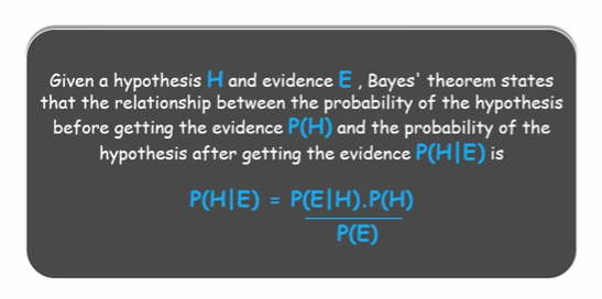
The Bayes theorem states that below:

Bayes Theory:

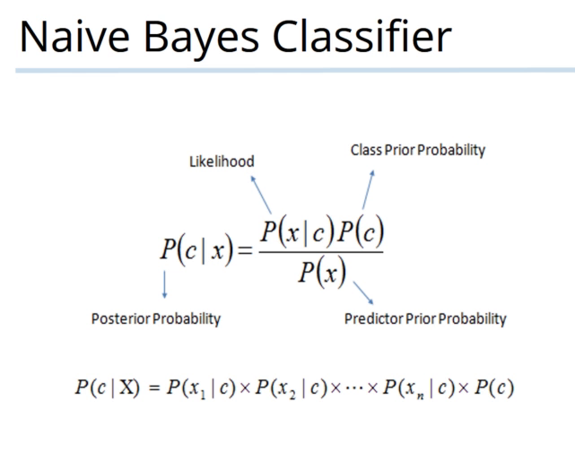
Naive Bayes theorem ignores the unnecessary features of the given datasets to predict the result. Many cases, Naive Bayes theorem gives more accurate result than other algorithms. The rules of the Naive Bayes Classifier Algorithm is given below:

Naive Bayes Classifier Formula:

Different Types Of Naive Bayes Algorithm:

1.  Gaussian Naive Bayes Algorithm – It is used to normal classification problems.
2.  Multinomial Naive Bayes Algorithm – It is used to classify on words occurrence.
3.  Bernoulli Naive Bayes Algorithm – It is used to binary classification problems.

Usage Of Naive Bayes Algorithm:

• News Classification.
• Spam Filtering.
• Face Detection / Object detection.
• Medical Diagnosis.
• Weather Prediction, etc.

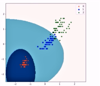
In this article, we are focused on Gaussian Naive Bayes approach. Gaussian Naive Bayes is widely used.

Let’s see how the Gaussian Naive Bayes Algorithm classifies the whole data by a suitable graph:

Classification Graph:

An Example of Naive Bayes theory

Lets we have a dataset of a Car Showroom:

Car data table:

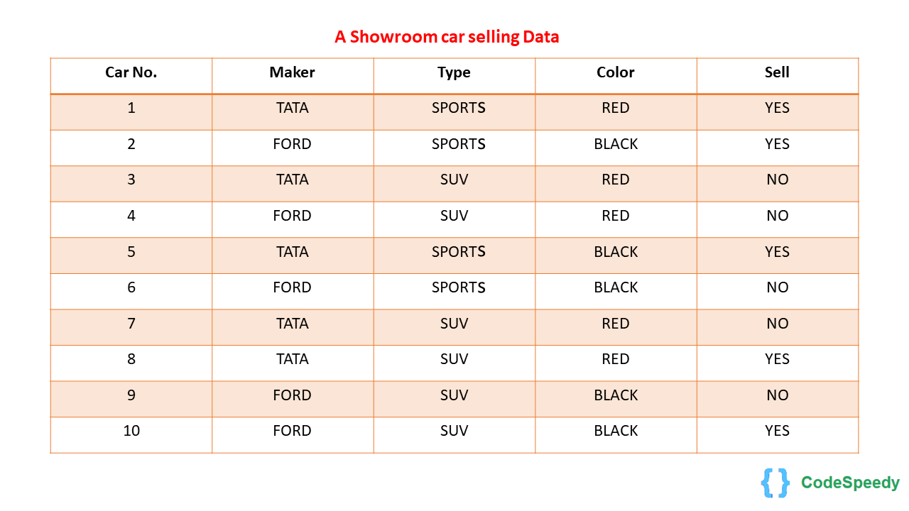
From the table we can find this :

P(YES) = 5/10
P(NO) = 5/10

Maker :

P(TATA|YES) = 3/5
P(FORD|YES) = 2/5

P(TATA|NO) = 2/5
P(FORD|NO) = 3/5

TYPE :

P(SPORTS|YES) = 3/5
P(SUV|YES) = 2/5

P(SPORTS|NO) = 1/5
P(SUV|NO) = 4/5

COLOR :

P(RED|YES) = 2/5
P(BLACK|YES) = 3/5

P(RED|NO) = 3/5
P(BLACK|NO) = 2/5

We want to find the result of a sample case of X.

Sample X = TATA SUV BLACK then, What will be the probability of sample X?

Solution:

The probability of YES:

P(X|YES).P(YES) = P(TATA|YES).P(SUV|YES).P(BLACK|YES).P(YES)

=> 3/5 . 2/5 . 3/5 . 5/10
=> 0.072

The probability of NO:

P(X|NO).P(NO) = P(TATA|NO).P(SUV|NO).P(BLACK|NO).P(NO)

=> 2/5. 4/5. 2/5. 5/10
=> 0.064

Here the Probability of “Yes” is high. The result will be “Yes”. This result is determined by the Naive Bayes algorithm.

Naive Bayes Algorithm in python

Let’s see how to implement the Naive Bayes Algorithm in python. Here we use only Gaussian Naive Bayes Algorithm.

Requirements:

1.  Iris Data set.
2. pandas Library.
3. Numpy Library.
4. SKLearn Library.

Here we will use The famous Iris / Fisher’s Iris data set. It is created/introduced by the British statistician and biologist Ronald Fisher in his 1936. The data set contains 50 samples of three species of Iris flower. Those are Iris virginica, Iris setosa, and Iris versicolor. Four features were measured from each sample: the sepals and petals, length and the width of the in centimetres.

It is widely used to train any classification model. So it is available on the sklearn package.

Let’s go for the code:

import pandas as pd
import numpy as np
from sklearn import datasets
iris = datasets.load_iris() # importing the dataset
iris.data # showing the iris data

Output:

array([[5.1, 3.5, 1.4, 0.2],
       [4.9, 3. , 1.4, 0.2],
       [4.7, 3.2, 1.3, 0.2],
       [4.6, 3.1, 1.5, 0.2],
       [5. , 3.6, 1.4, 0.2],
       [5.4, 3.9, 1.7, 0.4],
      .......
       [6.7, 3. , 5.2, 2.3],
       [6.3, 2.5, 5. , 1.9],
       [6.5, 3. , 5.2, 2. ],
       [6.2, 3.4, 5.4, 2.3],
       [5.9, 3. , 5.1, 1.8]])

Explain:

Here we import our necessary libraries. And import the iris dataset. And we print the data.

X=iris.data #assign the data to the X
y=iris.target #assign the target/flower type to the y

print (X.shape)
print (y.shape)

Output:

(150, 4)
(150,)

Explain:

Here we assign the features (data) of the flowers to the X variable. And the flower types(target) to the y variable. Then we print the size/shape of the variable X and y.

from sklearn.model_selection import train_test_split
X_train,X_test,y_train,y_test=train_test_split(X,y,test_size=0.2,random_state=9) #Split the dataset

Explain:

Here we split our data set into train and test as X_train, X_test, y_train, and y_test.

from sklearn.naive_bayes import GaussianNB
nv = GaussianNB() # create a classifier
nv.fit(X_train,y_train) # fitting the data

Output:

GaussianNB(priors=None, var_smoothing=1e-09)

Explain:

Here we create a gaussian naive bayes classifier as nv. And we fit the data of X_train,y_train int the classifier model.

from sklearn.metrics import accuracy_score
y_pred = nv.predict(X_test) # store the prediction data
accuracy_score(y_test,y_pred) # calculate the accuracy

Output:

1.0

Explain:

Here we store the prediction data into y_pred. And calculate the accuracy score. We got the accuracy score as 1.0 which means 100% accurate.

The whole code is available in this file: Naive bayes classifier – Iris Flower Classification.zip

You may also like to read:

• Prepare your own data set for image classification in Machine learning Python
• Fitting dataset into Linear Regression model
• Binary Classification using Neural Networks