Plotting different Confidence Intervals around Fitted Line using R and ggplot2

In this blog post, I’ll show that how we can plot different confidence intervals i.e., 90%, 95% or 99% around the fitted line in R using ggplot2 library.
Load libraries
library(tidyverse)
library(stargazer)
library(patchwork)
Load data
For this blog post, I’ll use the built in cars data set. The data set contains only 2 variables i.e., speed and distance.
data("cars")
glimpse(cars)## Rows: 50
## Columns: 2
## $ speed <dbl> 4, 4, 7, 7, 8, 9, 10, 10, 10, 11, 11, 12, 12, 12, 12, 13, 13, 13…
## $ dist <dbl> 2, 10, 4, 22, 16, 10, 18, 26, 34, 17, 28, 14, 20, 24, 28, 26, 34…Simple Linear Regression
At first, I’ll fit a simple linear regression model for distance against speed.
model <- lm(dist ~ speed, data = cars)
stargazer::stargazer(model, type = "text")##
## ===============================================
## Dependent variable:
## ---------------------------
## dist
## -----------------------------------------------
## speed 3.932***
## (0.416)
##
## Constant -17.579**
## (6.758)
##
## -----------------------------------------------
## Observations 50
## R2 0.651
## Adjusted R2 0.644
## Residual Std. Error 15.380 (df = 48)
## F Statistic 89.567*** (df = 1; 48)
## ===============================================
## Note: *p<0.1; **p<0.05; ***p<0.01- We can see a significant positive association between distance and speed.
- As the speed increases, the distance also increases.
Now, we want to visualize this fitted model. An easy way is that we can use the geom_smooth function of ggplot2 package to show a trend line of association between speed and distance. geom_smooth also provides a built in function to plot the confidence interval around the fitted line.
Note: 95% confidence interval is the default level. However, we can change the levels manually also.
Fitted line with 95% confidence level
p1 <- cars %>%
  ggplot(aes(x = speed, y = dist)) +
  geom_point(colour = "black") +
  geom_smooth(method = "lm", se = TRUE) +
  labs(title = "95% Confidence Interval") +
  theme_bw() +
  theme(plot.title = element_text(face = "bold",hjust = 0.5))

p1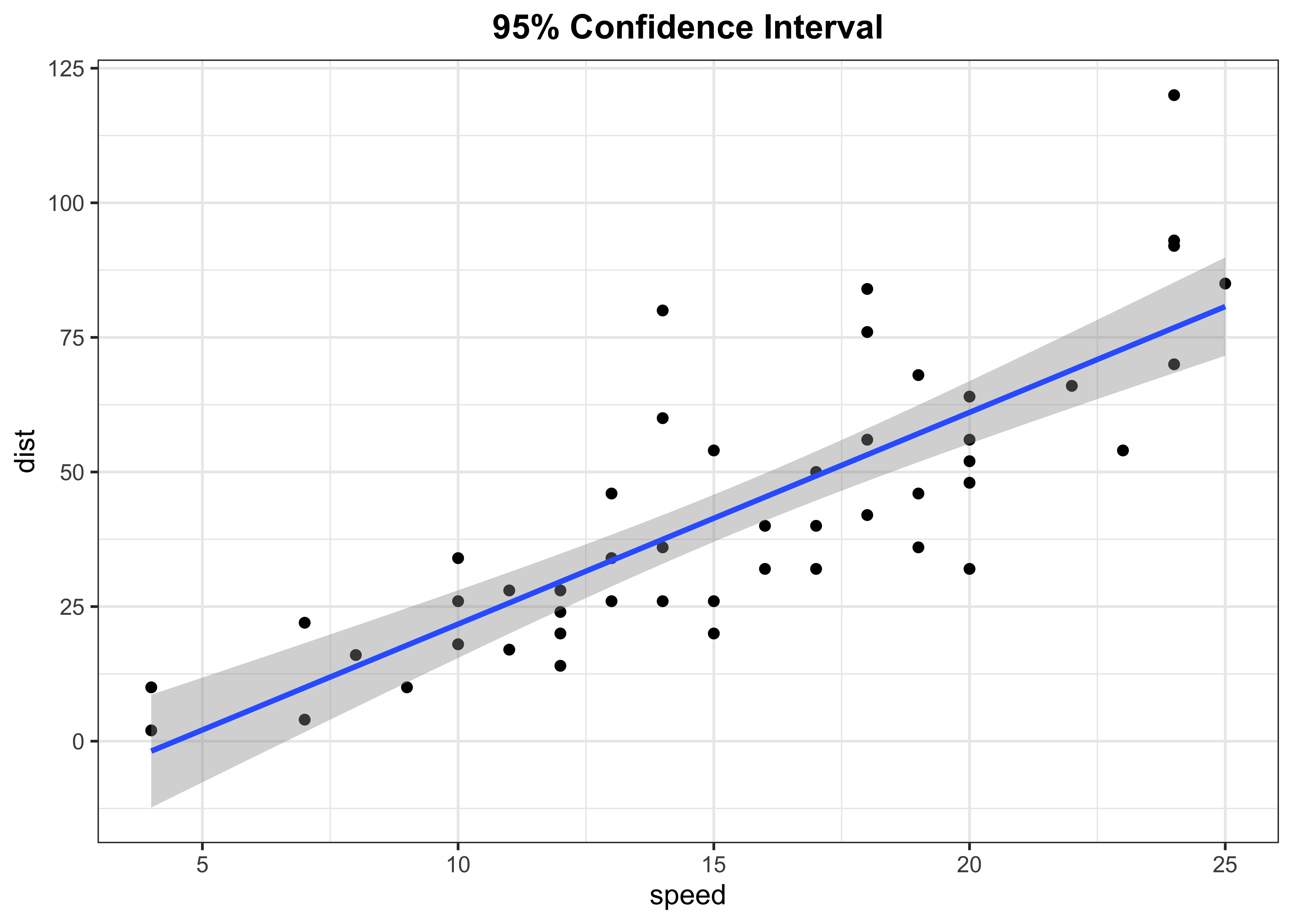
Fitted line with 90% confidence level
p2 <- cars %>%
  ggplot(aes(x = speed, y = dist)) +
  geom_point(colour = "black") +
  geom_smooth(method = "lm", se = TRUE, level = 0.90) +
  labs(title = "90% Confidence Interval") +
  theme_bw() +
  theme(plot.title = element_text(face = "bold",hjust = 0.5))

p2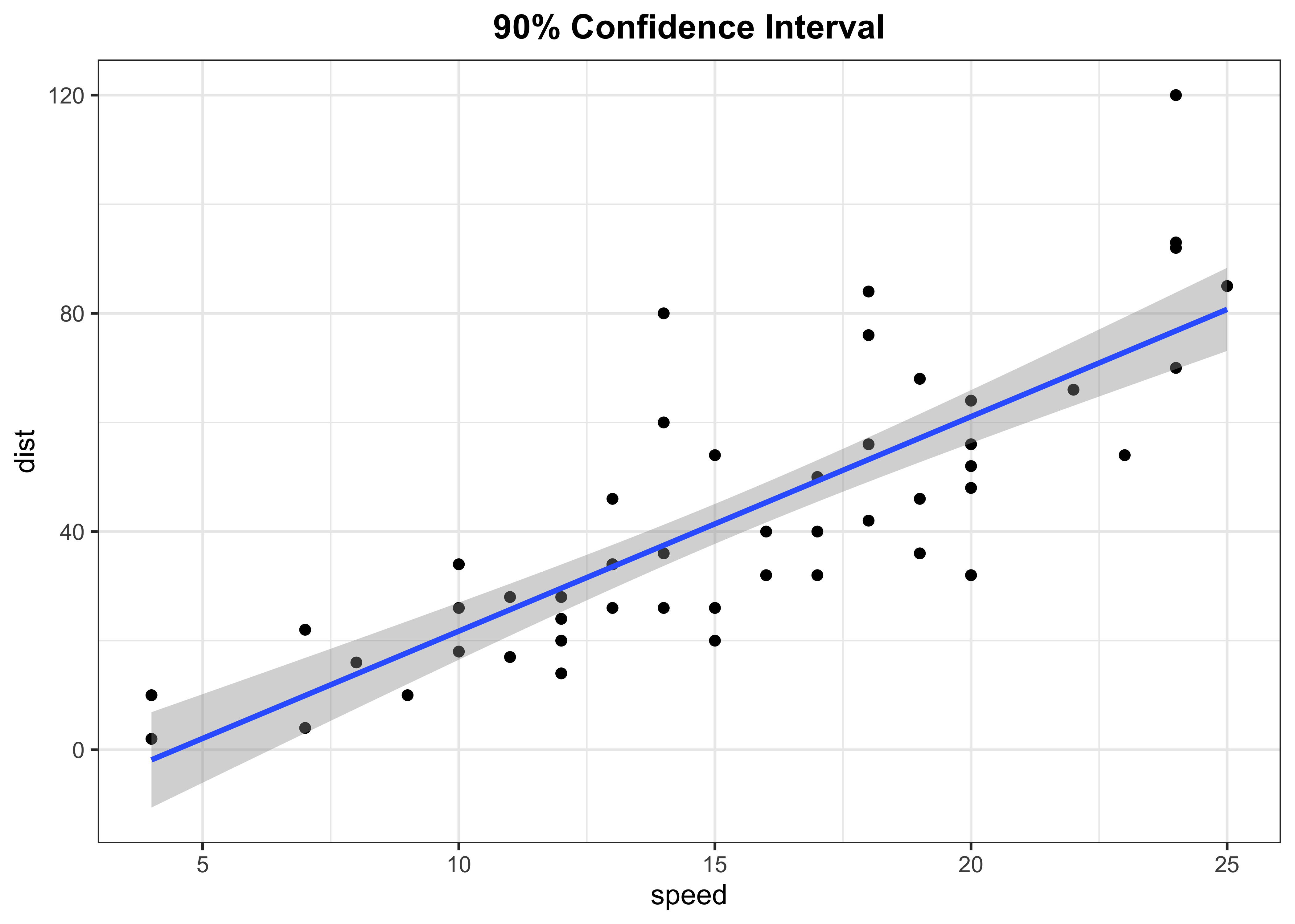
Fitted line with 90% confidence level
p3 <- cars %>%
  ggplot(aes(x = speed, y = dist)) +
  geom_point(colour = "black") +
  geom_smooth(method = "lm", se = TRUE, level = 0.99) +
  labs(title = "99% Confidence Interval") +
  theme_bw() +
  theme(plot.title = element_text(face = "bold",hjust = 0.5))

p3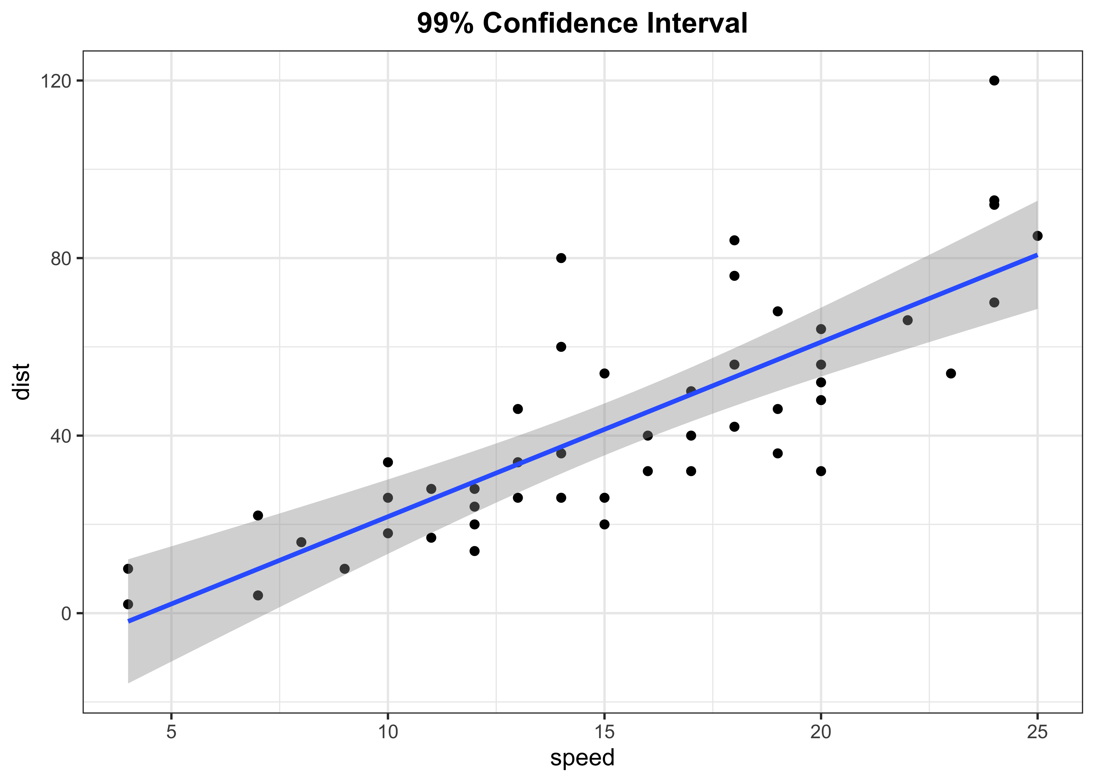
Stacking
p1 + p2 + p3 + plot_layout(ncol = 2)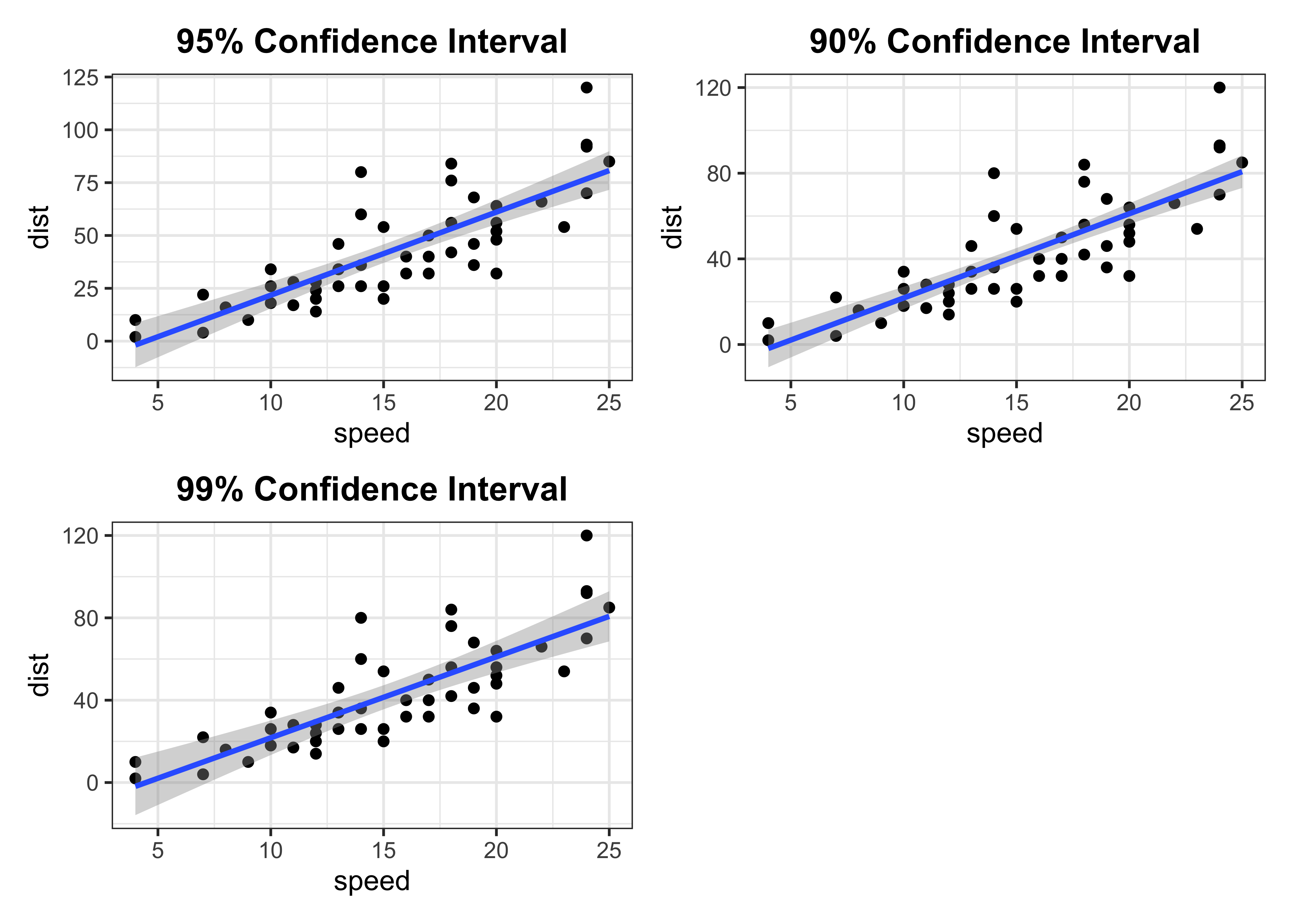
This is an easiest way to plot confidence intervals in R and ggplot2 even without fitting a regression model separately. However, sometime we want to compare different confidence interval bounds in a single scatter plot. In that case we need some creativity and extra lines of code. I know there can be different ways to achieve this but here is how I had accomplished this task.
- First, I’ll extract the confidence intervals of fitted line using the
predictfunction.
Extract confidence intervals data
# CI
ci90 <- predict(model, cars, interval = "confidence", level = 0.90)
ci95 <- predict(model, cars, interval = "confidence", level = 0.95)
ci99 <- predict(model, cars, interval = "confidence", level = 0.99)- After that, I’ll bind these data sets using the
bind_rowsfunction. Before binding, I’ll create an ID variable for eachdata.frameto keep track of the data.
# bind data
ci_pred <- as.data.frame(ci90) %>%
  mutate(ID = "90%") %>%
  bind_rows(as.data.frame(ci95) %>%
              mutate(ID = "95%"),
            as.data.frame(ci99) %>%
              mutate(ID = "99%")
              )

head(ci_pred)
## fit lwr upr ID
## 1...1 -1.849460 -10.591699 6.892779 90%
## 2...2 -1.849460 -10.591699 6.892779 90%
## 3...3 9.947766 3.050136 16.845396 90%
## 4...4 9.947766 3.050136 16.845396 90%
## 5...5 13.880175 7.563250 20.197100 90%
## 6...6 17.812584 12.050540 23.574627 90%- After that, I’ll join this data back with
carsdata usingbind_colsfunction followed by some data wrangling.
# Joining with cars data
final_data <- cars %>%
  bind_cols(
    ci_pred %>%
      remove_rownames() %>%
      pivot_wider(names_from = ID, values_from = c(lwr, upr)) %>%
      unnest()
  ) %>%
  pivot_longer(names_to = "key", values_to = "value", cols = 4:9) %>%
  separate(key, into = c("Type", "Level"), sep = "_") %>%
  pivot_wider(names_from = Type, values_from = value) %>%
  unnest()

head(final_data)
## # A tibble: 6 × 6
## speed dist fit Level lwr upr
## <dbl> <dbl> <dbl> <chr> <dbl> <dbl>
## 1 4 2 -1.85 90% -10.6 6.89
## 2 4 2 -1.85 95% -12.3 8.63
## 3 4 2 -1.85 99% -15.8 12.1
## 4 4 10 -1.85 90% -10.6 6.89
## 5 4 10 -1.85 95% -12.3 8.63
## 6 4 10 -1.85 99% -15.8 12.1- Now we have the cleaner data that contains fitted data along with confidence intervals at different levels.
- We can use this data to plot the confidence bounds around the fitted line in a single scatter chart.
Final Plot
final_data %>%
  ggplot(aes(x = speed, y = dist, color = Level)) +
  geom_point(colour = "midnightblue", alpha = 0.5) +
  geom_smooth(method = "lm", se = F, colour = "brown") +
  geom_line(aes(y = lwr), lty = 2) +
  geom_line(aes(y = upr), lty = 2) +
  labs(x = "Speed", y = "Distance", color = NULL) +
  theme_test() +
  theme(legend.position = c(0.08, 0.85))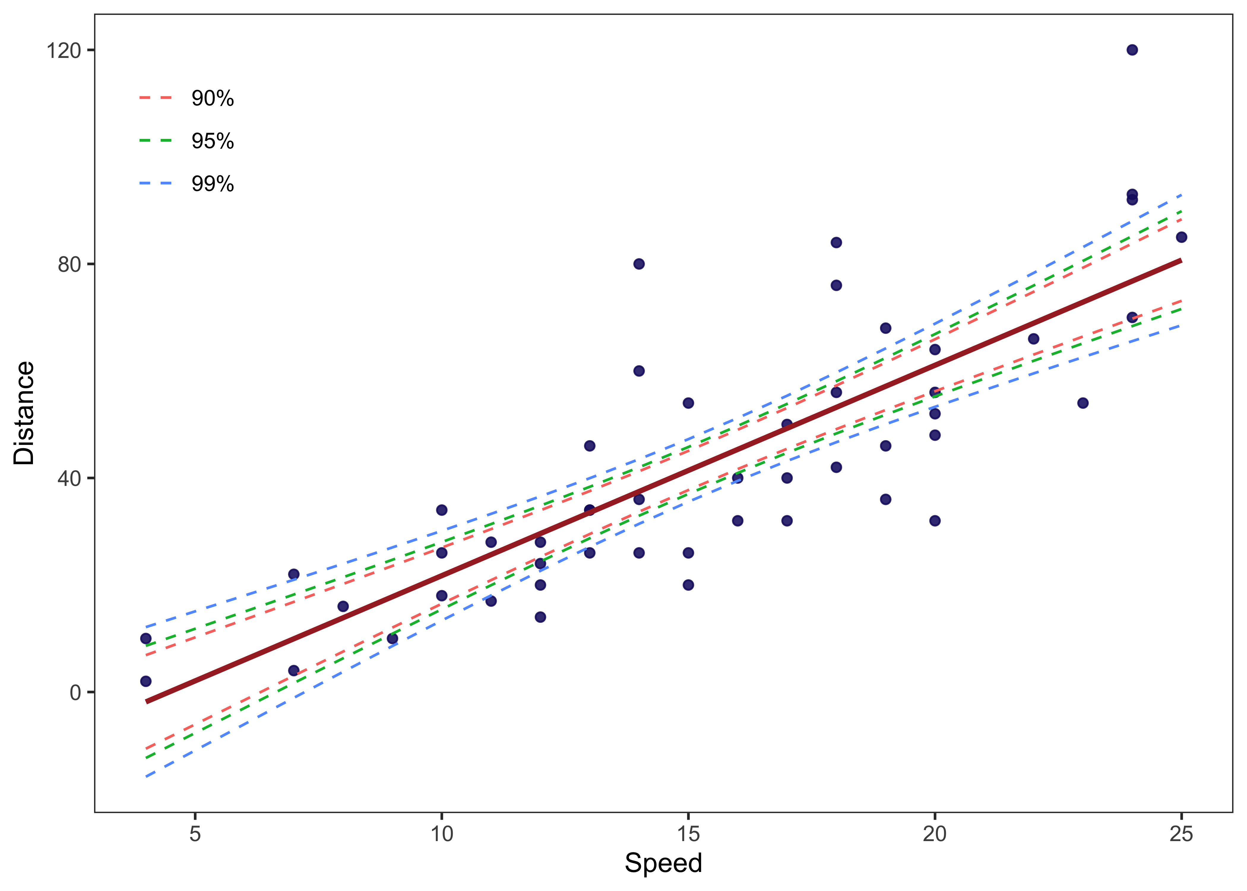
That’s it!
Feel free to reach me out if you got any questions.