Open In App

How to Wrap Text in Excel Automatically and Manually – 3 Easy Methods

Last Updated: 22 Nov, 2024
Summarize
Comments
Improve
Suggest changes
Like Article
Like
Save
Share
Report
News Follow

How to Wrap Around Text in Excel – Quick Steps

  • Select the cell(s).
  • Go to Home >> Click Wrap Text.
  • Adjust the row height if needed.

Wrapping text in Excel is a simple yet essential feature that ensures your data is displayed clearly and fits neatly within each cell. When working with long entries, such as names, addresses, or descriptions, text may overflow into adjacent cells or become hidden. This guide will show you how to wrap text in Excel, making your data more readable and organized. Whether you’re managing reports, creating tables, or formatting large datasets, wrapping text improves presentation and helps maintain a professional look.

How-to-Wrap-Text-in-Excel

How to Wrap Text in Excel

What Is Text Wrapping in Excel

Text wrapping in Excel adjusts the way text is displayed in a cell. Instead of text overflowing into adjacent cells or being cut off, wrapping breaks the text into multiple lines, fitting it neatly within the cell.

  • Example Without Wrapping: The text spills into adjacent cells or appears incomplete if the neighboring cell contains data.
  • Example With Wrapping: The text is displayed across multiple lines within the same cell.

Use Wrap Text Shortcut in Excel

Shortcuts are a quick way to apply text wrapping without navigating through menus.

Shortcuts:

  • Windows: Press Alt + H + W to apply text wrapping.
  • Mac: Use the Wrap Text button in the ribbon under the Home tab

How to Wrap Text in Excel Automatically (Windows & Mac)

Auto wrap text in Excel is a quick way to make long text fit within a cell without cutting it off. Here’s how you can do it on both Windows and Mac:

Method 1: Wrap Text Using the Ribbon (Wrap Text Button)

This method will help you to convert the long string into multiple lines. To force a lengthy text string to appear on multiple lines, select the cells that you want to format and turn on the Excel text wrap.

Follow the below steps to wrap text in Excel using Ribbon:

Step 1: Open Excel and Select Cell

Select the cell that you want to change.

Wrap Text in Excel

Open Excel

Step 2: Go Home Tab and Select Wrap Text

On the Home tab to the Alignment group and click Wrap Text. You will see that your entered text is now wrapped in the cell automatically.

Wrap Text in Excel

Go to the Home Tab >> Click on Wrap Text

Method 2: Wrap Text Using Format Cells

Follow the below steps to wrap text using the Format Cells dialog box:

Step 1: Select the Cell in which you have data

Select the cell that you want to change.

Wrap Text in Excel

Select the Cell

Step 2: Right Click and Select Format Cell

Right-click on it and click on the Format cell in the drop down menu.
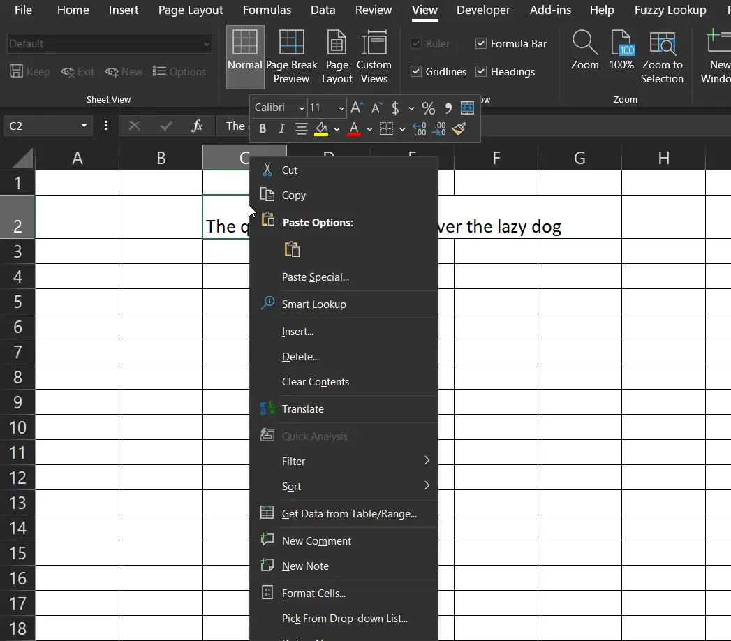
Wrap Text in Excel

Perform a Right-click >> Select Format Cells
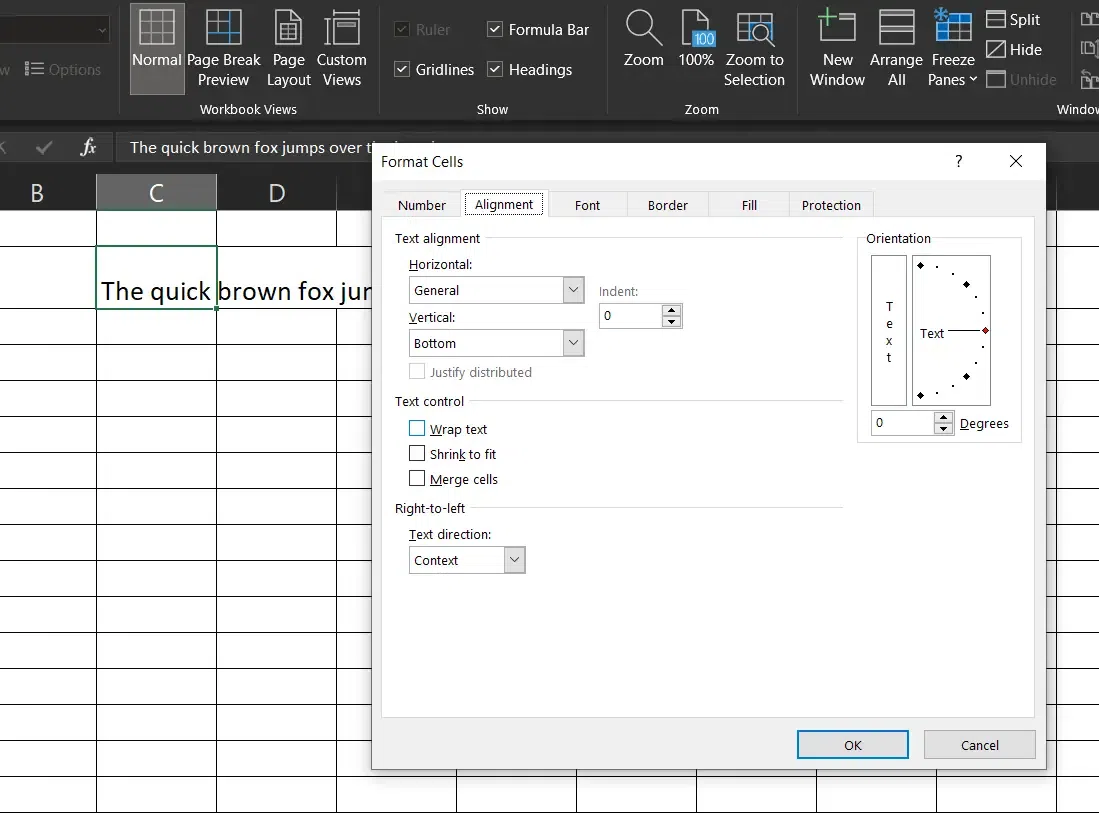
Step 3: Select Alignment in the Format Cells Dialog Box.

Wrap Text in Excel

Select Alignment Tab

Step 4: Check Wrap Text in the Text Control Option and click OK.

Wrap Text in Excel

Check Wrap Text >> Click “Ok”

Method 3: Using the Keyboard Shortcut

Follow the below steps to wrap text in Excel using keyboard shortcut:

Step 1: Open Excel and Select Cell

Select the cell that you want to change.

Wrap Text in Excel

Select a Cell

Step 2: Press ALT, H and W

Press Alt + H + W on your keyboard.
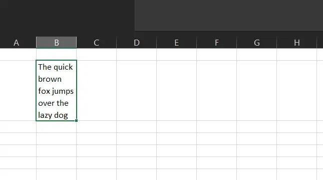
Wrap Text in Excel

Press Alt + H +W

How to Wrap Text in Excel Manually with Line Breaks

If you want more control over where the text wraps, you can insert manual line breaks.

Step 1: Enter Edit Mode

Double-click the cell or press F2 to edit the text.

Wrap Text in Excel

Select the Cell

Step 2: Insert Line Breaks

Place the cursor where you want the text to break into a new line. Press Alt + Enter (Windows) or Option + Return (Mac).

Wrap Text in Excel

Place the Cursor

Step 3: Enable Wrap Text

Ensure the Wrap Text feature is turned on under the Home tab.

Wrap Text in Excel

Press Alt + Enter

How to Unwrap Text in Excel using Right Click

Follow the below steps to remove wrap text using the format cells dialog box:

Step 1: Select the Cell

Select the cell that you want to change.

Wrap Text in Excel

Select the Text

Step 2: Right Click on the Cell and Select Format Cells

Right-click on Cell and click on the Format cell on the Dialog Box.

Wrap Text in Excel

Right-click on the Cell >> Click on Format Cell

Step 3: Choose Alignment

Select Alignment in the Format Cells Dialog Box.
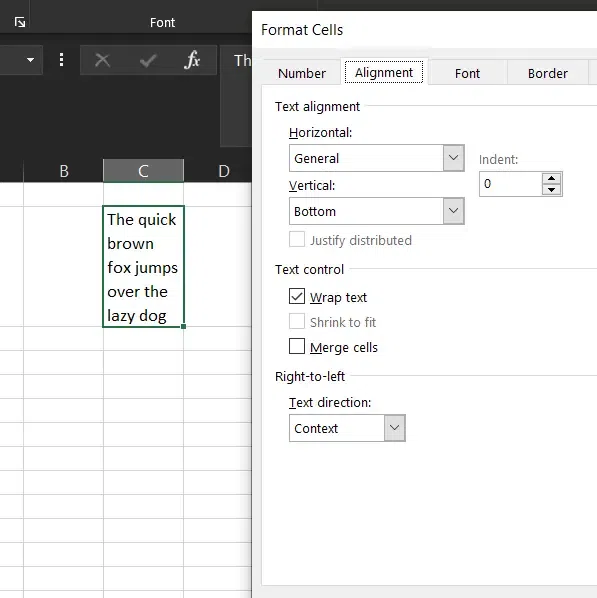
Wrap Text in Excel

Select Alignment Cells

Step 4: Uncheck Wrap Text and Click ok

Uncheck Wrap Text in the Text Control option and click OK.
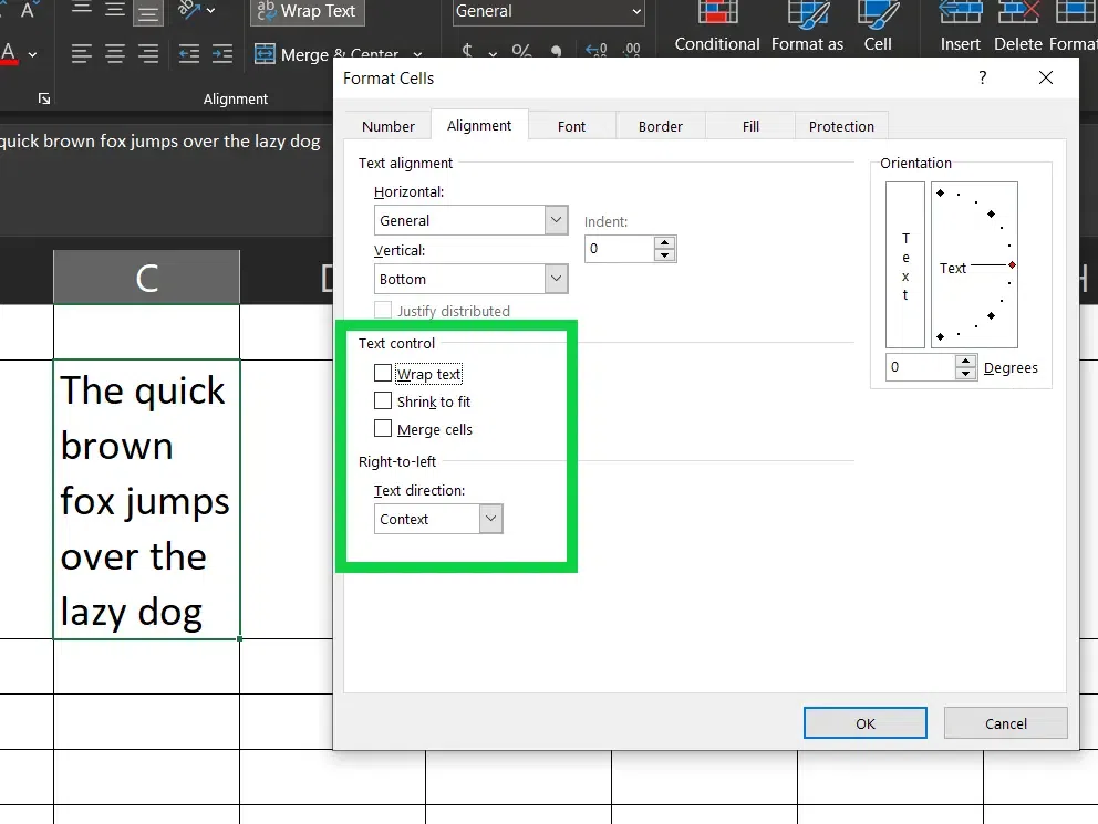
Wrap Text in Excel

Uncheck the Wrap Text >> Click “Ok”

Alternatively, press the “Ctrl+1” shortcut to open the Format cells dialog and clear the Wrap Text check box on the alignment tab.

Troubleshooting Common Text Wrapping Issues

1. Wrapped Text Doesn’t Fit

Problem: Text appears cut off even after enabling wrapping.

Solution:

  • Adjust the row height by dragging the bottom edge of the row number.
  • Use AutoFit Row Height by double-clicking the bottom border of the row number.

2. Wrap Text Doesn’t Work

Problem: The text remains in one line despite applying wrap text.

Solution:

  • Ensure the cell is not merged, as merged cells often conflict with text wrapping.
  • Use the Format Cells method to ensure the wrap text setting is applied.

3. Column Width Limits

Problem: Wrapped text becomes unreadable due to narrow columns.

Solution:

  • Adjust column width to improve readability.
  • Combine wrapping with vertical alignment for better aesthetics.

Conclusion

Mastering how to text wrap in Excel is an essential skill for anyone working with spreadsheets. Whether you’re managing data, creating reports, or formatting Google Sheets, understanding how to use this feature will save you time and make your work look professional. By following these methods—using the ribbon, shortcuts, or format cells—you can efficiently organize and display long text within your Excel sheets.

How to Wrap Text in Excel Automatically and Manually – FAQs

How to Wrap Text in Google Spreadsheet

You can also go to Format > Text wrapping > Wrap to apply this setting.

Where Is Wrap Text in Excel?

The Wrap Text option is located in the Home tab under the Alignment group. It’s represented by an icon showing text in a cell broken into lines. This is where you apply, disable, or modify text wrapping.

How do you Get text to Wrap in Excel?

Select the Cell(s): Highlight the cell or range of cells where you want the text to wrap.

  • Enable Wrap Text:
  • Go to the Home tab.
  • Click the Wrap Text button in the Alignment group.

Adjust Row Height (if needed):

  • Excel will automatically adjust the row height to fit the wrapped text.
  • You can also manually adjust the row height by dragging the row border.

How to wrap text in merged cells in Excel?

To Wrap Text in Merged cells in Excel, Follow the below steps:

Step 1: Select the Merged Cell(s)

Highlight the merged cell or range of merged cells where you want to wrap text.

Step 2: Enable Wrap Text

Go to the Home Tab → In the Alignment group, click on Wrap Text.

Step 3: Adjust Row Height (if needed)

Excel doesn’t automatically adjust the row height for merged cells.

Manually drag the row border to increase the height and display all the wrapped text.

How to Fit Long text in a Single Cell with Multiple Lines in Excel?

Fit Long Text in a Single Cell with Multiple Lines in Excel

  • Select the Cell: Click on the cell where you want the text.
  • Enable Wrap Text: Go to Home → Click Wrap Text in the Alignment group.
  • Add Line Breaks (if needed): Press Alt + Enter (Windows) or Option + Enter (Mac) to insert a line break manually.
  • Adjust Row Height: Drag the row border to fit the text, or let Excel adjust it automatically.

This ensures long text fits neatly within a single cell on multiple lines.

Where is Wrap Text in Excel?

You can find the Wrap Text option in the Home Tab under the Alignment group. Alternatively, you can use the Format Cells dialog or shortcuts for quick access.

How Do I Wrap Text in Google Spreadsheet?

Go to Format >>Text Wrapping >>Wrap to enable wrapping in Google Sheets.

Why can’t I wrap text in Excel?

Here are some common causes which can be a issue:

  • Cell Format
  • Merged Cells
  • Cell Size
  • Hidden Columns or Rows

How to wrap text in excel over multiple cells?

To wrap text in multiple cells simultaneously follow the below steps:

Step 1: Select the range of cells you want to wrap text in.

Step 2: Right-click and go to the “Format cells”, and enable “Wrap text”.

How to wrap text in Excel mac?

Here are some steps by which you can wrap text in Excel Mac:

  • Open Your Excel Spreadsheet
  • Select the Cells
  • Go to the Home Tab
  • Wrap Text Option
  • Adjust Row Height

How Do I Wrap Text in Excel Shortcut?

Press Alt + H + W (Windows) or Option + Command + W (Mac) to enable text wrapping instantly.

How do I wrap text in a cell size in Excel?

Here are some steps to wrap text in a cell size in Excel:

  • Open Your Excel Spreadsheet
  • Select the Cells
  • Go to the Home tab
  • Press Alt + H, then W


News
Improve
Discuss

How to Expand Cells to Fit the Text Automatically in Excel?

article_img
We all know how useful Excel is to store tabular data. We can do calculations in excel, we can store any information that is in the form of tables, and so on. But there are some common problems that we all face while using Excel. One of the problems that we encounter while entering oversized, overlength data in a cell. Whenever we enter any data that is not fitted in the cell every time we need to resize the column width and that is too frustrating. This article will show you how to make your cells automatically change their width whenever any oversized data is entered. Steps to make Rows/Columns Fit Text Automatically in Excel Initially, we have a table with column names “Name” and “Address". When we enter the data in the cells the data does not get fully fitted in the cells. Now, let's look at the steps to be followed: Step 1: Right-click on the sheet name in the bottom-left corner. Step 2: Now select “View Code”. Step 3: Select “Worksheet” from the drop-down menu as shown in the image. Step 4: You will see a console window with some code. Now, Enter the below code of the line in the console on the second line. Cells.EntireColumn.AutoFit Now close the window from the file menu. S
Read More

How to Compare Two Columns in Excel : Easy and Quick Methods

article_img
In the world of data analysis, knowing how to compare two columns in Excel is a fundamental skill that can unveil valuable insights and ensure data accuracy. If you're looking to spot differences, find duplicates, or identify similarities, mastering Excel's compare columns functionality is key. This article will walk you through effective methods on how to compare two columns in Excel, exploring techniques to streamline your workflow and make informed decisions. By the end, you'll be equipped with the knowledge to confidently manage and analyze your data using Excel compare two columns features. Let's explore and learn the power of data comparison! Table of Content Why Compare Two Columns in ExcelHow to Compare Two Columns in ExcelCompare Two Columns in Excel using Conditional FormattingHighlight Unique DataCompare Two Columns in Excel Using Equals OperatorCompare Two Columns in Excel Using the IF Condition Using the Lookup Function to Compare Two ColumnsWhy Compare Two Columns in ExcelExcel is a versatile tool that stores data and manipulates data for better decision-making. We are required to compare Excel columns data for the following reasons: To find the unique value in the da
Read More

How to Separate First and Last Name in Excel: 3 Easy Methods

article_img
How to Split Names in Excel - Quick StepsOpen MS Excel>>Select the ColumnOpen Text to Columns WizardChoose Delimited>>Select DelimitersSet Destination>>Adjust ColumnsManaging datasets with full names in a single column can be challenging when you need the names split into first and last names. Knowing how to separate first and last names in Excel is a practical skill that improves data clarity and organization. Whether you're working on a mailing list, a contact sheet, or any dataset requiring distinct name columns, Excel offers straightforward solutions. Using tools like Text to Columns, Flash Fill, Excel formulas or formulas like LEFT, RIGHT, and SEARCH, you can effortlessly break names into individual components. This guide will walk you through step-by-step methods to split names in Excel, saving time and ensuring your data is well-structured and ready for analysis. Table of Content How to Separate Names in Excel: 3 MethodsMethod 1: How to Split Names in Excel Using Text to ColumnsMethod 2: How to Separate First and Last Name in Excel with FormulasMethod 3: How to Split Names in Excel Using Flash FillHow to Split Full Name into First, Last, and Middle Name in
Read More

How to Split Cells in Excel: Easy Methods Explained

article_img
How to Separate a Cell in Excel- Quick StepsOpen MS Excel>>Select Data Go to the Data tab>>Click Text to Columns.Choose Delimited and click NextSplitting cells in Excel can simplify data management, especially when dealing with combined information in a single column or cell. Whether you’re separating names, dates, or other data points, understanding how to split cells in Excel is essential for better organization and clarity. This guide will show you how to break up cells in Excel using different methods. By the end, you'll know how to split cells horizontally, divide a cell in Excel for better Management. Table of Content What Does Splitting Cells in Excel MeanHow to Split Cells in Excel Using Text to Columns - 2 MethodsHow to Split Cells in Excel Using FormulasHow to Split Cells in Excel Using Flash Fill - 2 MethodsHow to Split Cells in Excel Using Power QueryHow to Divide a Cell in Excel in Excel Using Text Functions in ExcelCommon Use Cases for Splitting Cells in ExcelWhat Does Splitting Cells in Excel MeanSplitting a cell in Excel involves dividing its content into multiple cells or columns. For instance, you can: Separate first and last names.Break product catego
Read More

How to Insert Multiple Rows in Excel: 4 Easy Methods

article_img
How to Add Multiple Rows in ExcelSelect Rows >> Highlight the same number of rows you want to insert.Insert Rows >> Right-click and choose Insert.If you're looking to insert multiple rows in Excel quickly and without hassle, you're in the right place. Whether you're working with a simple table or a complex dataset, knowing how to add multiple rows in Excel is an essential skill. In this guide, we'll walk you through four easy methods to insert multiple rows at once. From using keyboard shortcuts to using the Insert option, copy-pasting, or even using the Name Box regardless of whether you're using Windows or Mac, these techniques will help you save time and keep your data organized. Table of Content How to Insert Multiple Rows in Excel using the Insert OptionHow to Insert Multiple Rows using an Excel ShortcutHow to Insert Multiple Rows using the Copy and Paste MethodHow to Insert Multiple Rows Using Name BoxHow to Insert Multiple Rows in Excel using the Insert OptionIf you are searching how to insert more than one row in excel between data automatically then adding rows using the Insert option would be the best method, This method is simple and effective for quickly add
Read More

How to Start a New Line in Excel Cell: 4 Easy Methods

article_img
How to Insert a Line Break in a Cell- Quick Steps Click on Cell >> Press F2Press "Alt+ Enter" to Create a new Line Press Enter Starting a new line within a cell in Excel can be incredibly useful when you want to enter multiple pieces of information or data in a single cell without cluttering your spreadsheet. Whether you're organizing addresses, adding comments, or formatting text for readability, knowing how to create a new line within a cell helps you maintain a clean and structured look. Fortunately, Excel makes this easy to do. In this guide, you'll learn how to start a new line in an Excel cell using a simple keyboard shortcut or a formula, allowing you to customize your spreadsheet with ease. Table of Content Method 1: Using Keyboard Shortcut in ExcelMethod 2: How to Create a New line in Excel cell Using FormulaMethod 3: Multiple Line Breaks in ExcelMethod 4: Line Break After a Specific Character in ExcelMethod 1: Using Keyboard Shortcut in ExcelTo start a new line of text or add spacing between lines or paragraphs of text in a worksheet cell, press Alt+Enter to insert a line break. To quickly insert a line break in Excel on both Windows and Mac, you can use the followi
Read More

How to Compare Two Lists in Excel: 5 Easy Methods

article_img
Comparing two lists in Excel is a powerful way to identify matches, differences, or duplicates within your data. Whether you’re working with inventory records, customer databases, or project tasks, knowing how to compare two lists in Excel can save time and improve accuracy. Excel offers several tools for this purpose, such as formulas like VLOOKUP, IF, as well as conditional formatting. This guide will walk you through step-by-step methods to effectively compare two lists in Excel, ensuring you can analyze your data quickly and efficiently. Table of Content Why Compare Two Lists in ExcelHow to Compare two Lists in Excel : 5 Different MethodsMethod 1: Using Conditional Formatting Method 2: Using the Equal Sign Operator Method 3: Using VLOOKUP Formula Method Method 4: Using Row Difference Method 5: Using IF ConditionWhy Compare Two Lists in ExcelComparing two lists is essential for tasks like: Identifying missing or duplicate entries.Validating records between two databases.Analyzing differences in inventory, sales, or employee datasets.Excel offers versatile tools to help you achieve these objectives with ease. How to Compare two Lists in Excel : 5 Different MethodsWhen working wit
Read More

How to Create a Drop-Down List in Excel : 2 Easy Methods

article_img
How to make a Drop-Down List in Excel: Quick StepsOpen MS Excel Spreadsheet >> Enter List Items Select Cell >> Go to Data Validation Choose List Option Set the Source >>Click OKA drop-down list in Excel is an essential tool that simplifies data entry and helps maintain consistency across your spreadsheets. It allows users to select from a predefined set of options, reducing the risk of errors and speeding up the input process. This guide will show you how to create an Excel pull-down list using existing data, as well as more advanced techniques, such as creating dynamic drop-down lists that automatically update. We’ll also explore how to use formulas like OFFSET and UNIQUE to create flexible and dynamic drop-down lists, which can adapt to changing data. Additionally, we will guide you through customizing input messages and error alerts to make your lists even more user-friendly. Table of Content How to Create a Drop-Down List in Excel (2 Methods)Method 1: Creating a Drop-Down List for An Already Existing Data Method 2: Manually Creating a Custom Drop-Down List in ExcelHow to Create a Dynamic Drop-Down List in Excel (2 Methods)Method 1: Creating a Dynamic Dependent
Read More

How to Unprotect a Sheet in Excel (5 Easy Methods)

article_img
Have you ever come across an Excel sheet that's locked, stopping you from making changes or updates? Whether it’s to prevent accidental changes or to keep sensitive information safe, sometimes you need to remove that protection to get back to editing. If you're wondering how to break Excel sheet protection, you're in the right place. Fortunately, unprotecting an Excel sheet is easier than you might think. In this guide, we’ll show you 5 simple methods to unprotect a sheet in Excel, whether you’re using the latest version like Excel 365 or an older one like Excel 2010. We’ll cover everything from built-in options like the Review Tab and Right-click, to using Google Sheets and even a bit of VBA coding for those who need more advanced solutions. Table of Content What Does Unprotecting a Sheet Mean in ExcelMethod 1: Unprotect Sheet Using the Built-In OptionMethod 2: Unprotect a Sheet by Right-Clicking on the Sheet TabMethod 3: Unlock Excel Sheets Using VBA Code (For Excel 2010 and Earlier Versions)Method 4: Use Online Tools to Remove Protection from Excel SheetsMethod 5: Unlock Excel Sheets by Uploading to Google SheetsWhat Does Unprotecting a Sheet Mean in ExcelUnprotecting a sheet in
Read More

How to Make a Histogram in Excel: 3 Easy Methods

article_img
A histogram is a vital tool for analyzing and visualizing the distribution of data, allowing users to easily identify patterns, trends, and outliers. Commonly used in statistics and data-driven decision-making, histograms help present data frequency in a structured and readable format. Excel provides multiple ways to create histograms, catering to different versions and user preferences. In this guide, you’ll learn how to make a histogram in Excel using three methods: the built-in Histogram Chart for Excel 2016 and later, the Data Analysis ToolPak for earlier versions, and creating a Frequency Chart in Excel using formulas. Disclaimer: Always double-check your data for accuracy to ensure precise and reliable results. Method 1: Using the Built-in Histogram Chart (Excel 2016 and Later)For Excel 2016 and later versions, a Histogram Chart is available as a built-in feature. Follow the below step by step process to make a histogram chart in excel: Step 1: Prepare Your DataOrganize your data in a single column. For example: Here we have Test scores of a Student: Step 2: Insert a HistogramSelect the data range (e.g., A2:A8).Go to the Insert tab.In the Charts group, click Insert Statistic
Read More
three90RightbarBannerImg